Foundation details about Modelling Data (PL-300)

Titbits of Information about Model data with Power BI from the Learning Path

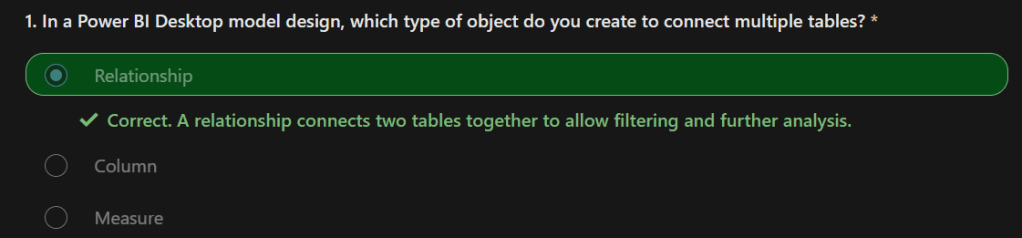
1. Understanding the structure of semantic models can help you design the right model to support your reports and dashboards.

A semantic model can be developed in many ways, yet one or several of those ways are more optimal. Optimal models are important for delivering good query performance and for minimizing data refresh times and the use of service resources, including memory and CPU.

The fewer resources that are used, the more models that can be hosted and at lower cost.

2. A single-table model can be a simple design, perhaps one that’s suitable for a data exploration task or proof of concept, but not one that’s an optimal model design.

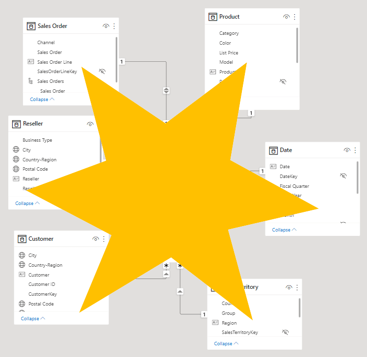
3. An optimal model adheres to star schema design principles. Star schema refers to a design approach that’s commonly used by relational data warehouse designers because it presents a user-friendly structure and it supports high-performance analytic queries.

4. This design principle is called a star schema because it classifies model tables as either fact or dimension. In a diagram, a fact table forms the center of a star, while dimension tables, when placed around a fact table, represent the points of the star.

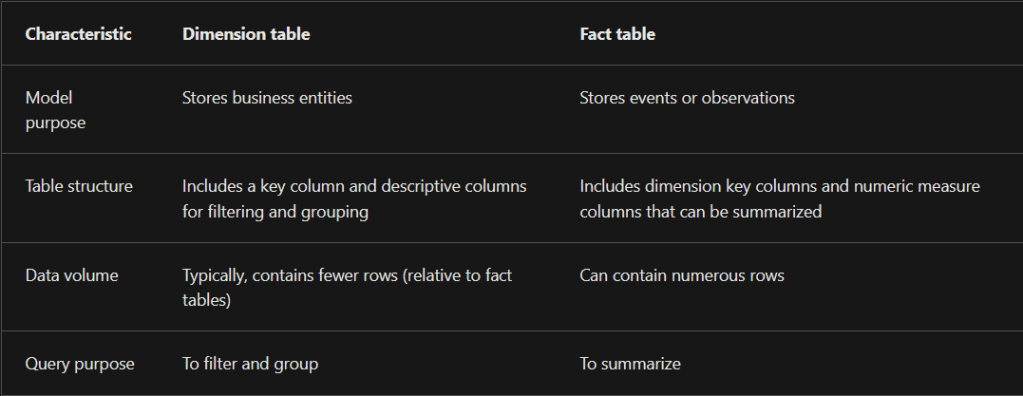
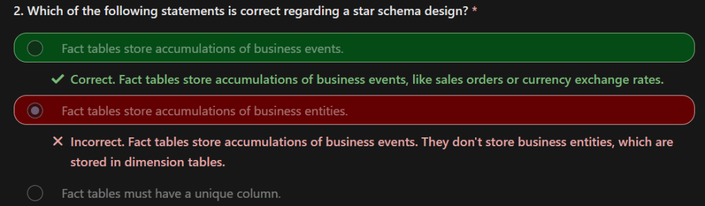
5. The role of a fact table is to store an accumulation of rows that represent observations or events that record a specific business activity. For example, events that are stored in a sales fact table could be sales orders and the order lines. You could also use a fact table to record stock movements, stock balances, or daily currency exchange rates. 

6. Generally, fact tables contain numerous rows. As time passes, fact table rows accumulate. In analytic queries (which will be defined later in this module), fact table data is summarized to produce values like sales and quantity.

7. Dimension tables describe your business entities, which commonly represent people, places, products, or concepts. A date dimension table, which contains one row for each date, is a common example of a concept dimension table. The columns in dimension tables allow filtering and grouping of fact table data.

8. Each dimension table must have a unique column, which is referred to as its key column.

9. A unique column doesn’t contain duplicate values and it should never have missing values. In a product dimension table, the column could be named ProductKey or ProductID

10. Fact vs Dimension

11. dimension tables are related to fact tables by using one-to-many relationships. The relationships allow filters and groups that are applied to dimension table columns to propagate to the fact table. This design pattern is common.

12. Dimension tables can be used to filter multiple fact tables, and fact tables can be filtered by multiple dimension tables. However, it’s not a good practice to relate a fact table directly to another fact table.

13.

14. An analytic query is a query that produces a result from a semantic model. Each Power BI visual, in the background, submits an analytic query to Power BI to query the model. 

15.  The analytic query is written as a Data Analysis Expressions (DAX) query statement. However, you don’t need to write a native DAX statement; you only need to configure report visuals by mapping semantic model fields.

16. An analytic query has three phases that are implemented in the following order:

1. Filter
2. Group
3. Summarize

17. Filtering – Filtering, or slicing, targets the data of relevance. In Power BI reports, filters can be applied to three different scopes: the entire report, a specific page, or a specific visual. Filtering is also applied in the background when row-level security (RLS) is enforced. Each report visual can inherit filters or have filters directly applied to it.

18. Grouping, or dicing, divides query results into groups.

19. Summarizing produces a single value result. Typically, numeric columns are summarized by using summarization methods (sum, count, and many others). These methods are simple summarizations. More complex summarizations, like a percent of grand total, can be achieved by defining measures that are written in DAX.

20. Not all analytic queries need to filter, group, and summarize:

• Commonly, report visuals are filtered, perhaps by a time period or geographic location.
• Grouping is optional. For example, a card visual, which is used to display a single value, isn’t concerned with grouping.
• Typically, report visuals summarize. One notable exception, however, is the slicer visual, which isn’t concerned with summarization.

21. Configure report visuals – Report authors produce report designs by adding report visuals and other elements to pages. Other elements include text boxes, buttons, shapes, and images. Each of these elements is configured independently of semantic model fields.

22. adding and configuring a report visual involves the following methodology

1. Select a visual type, like a bar chart.
2. Map semantic model fields, which are displayed in the Fields pane, to the visual field wells. For a bar chart, the wells are Y-axis, X-axis, Legend, Small multiples, and Tooltips.
3. Configure mapped fields. It’s possible to rename mapped fields or toggle the field to summarize or not summarize. If the field summarizes, you can select the summarization method.
4. Apply format options, like axis properties, data labels, and many others.

23. The following example shows how to configure the analytic query for a report visual. 

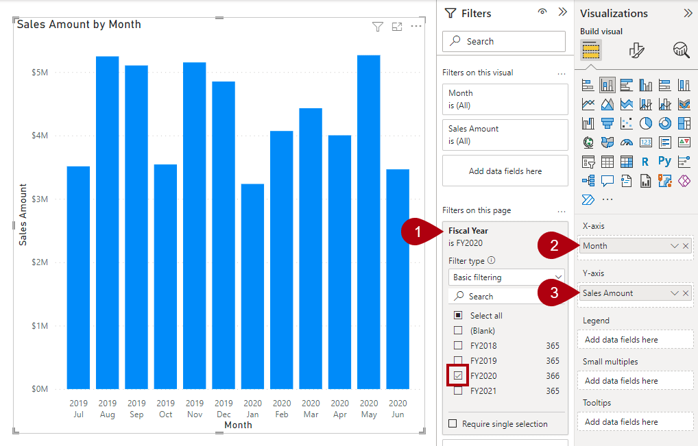
1. Add a stacked column chart visual to the report page.
2. Filter the page by using Fiscal Year from the Date table and selecting FY2020.
3. Group the visual by adding Month from the Date table to the X-axis well.
4. Summarize the visual by adding Sales Amount from the Sales table to the Y-axis well.

24. Fields is a collective term that is used to describe a model resource that can be used to configure a visual. The three different model resources that are fields include:

• Columns
• Hierarchy levels
• Measures

25. Filter vs Group vs summarize

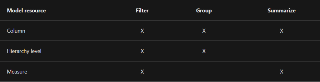
26. Use columns to filter, group, and summarize column values.

• Summarizing numeric columns is common, and it can be done by using sum, count, distinct count, minimum, maximum, average, median, standard deviation, or variance.
• You can also summarize text columns by using first (alphabetic order), last, count, or distinct count.
• Additionally, you can summarize date columns by using earliest, latest, count, or distinct count.

27. Year column should not be summarised –  If your semantic model has a numeric column that stores year values, it would be appropriate to set its default summarization to Do not summarize because the column will likely be used only for grouping or filtering, and that numeric summarization of years, like an average, doesn’t produce a meaningful result.

28. While hierarchy levels are based on columns, they can be used to filter and group but not to summarize. Report authors can summarize the column that the hierarchy level is based on, provided that it’s visible in the Fields pane.

29. Measures are designed to summarize model data; they can’t be used to group data. However, measures can be used to filter data in one special case: to use a measure to filter a visual when the visual displays the measure and the filter is a visual-level filter (so, not a report or page-level filter).

30. measures can be used to filter data in one special case: to use a measure to filter a visual when the visual displays the measure and the filter is a visual-level filter (so, not a report or page-level filter). 

31.

32.

33. For over two decades, Microsoft continues to make deep investments in enterprise business intelligence (BI). Azure Analysis Services (AAS) and SQL Server Analysis Services (SSAS) are based on mature BI data modeling technology used by countless enterprises. The same technology is also at the heart of Power BI data models.

34. Important terms in Power BI

• Data model
• Power BI dataset
• Analytic query
• Tabular model
• Star schema design
• Table storage mode
• Model framework

35. A Power BI data model is a query-able data resource that’s optimized for analytics. Reports can query data models by using one of two analytic languages: Data Analysis Expressions (DAX) or Multidimensional Expressions (MDX).

36. Power BI uses DAX, while paginated reports can use either DAX or MDX. The Analyze in Excel features uses MDX.

37. You develop a Power BI model in Power BI Desktop, and once published to a workspace in the Power BI service, it’s then known as a dataset. A dataset is a Power BI artifact that’s a source of data for visualizations in Power BI reports and dashboards.

38. Power BI reports and dashboards must query a dataset. When Power BI visualizes dataset data, it prepares and sends an analytic query. An analytic query produces a query result from a model that’s easy for a person to understand, especially when visualized.

39. Filtering (sometimes known as slicing) narrows down on a subset of the model data. Filter values aren’t visible in the query result. 

40. Grouping (sometimes known as dicing) divides query result into groups. Each group is also a filter, but unlike the filtering phase, filter values are visible in the query result. For example, grouping by customer filters each group by customer.

41. Summarization produces a single value result. Typically, a report visual summarizes a numeric field by using an aggregate function. Aggregate functions include sum, count, minimum, maximum, and others. You can achieve simple summarization by aggregating a column, or you can achieve complex summarization by creating a measure using a DAX formula.

42. A Power BI model is a tabular model. A tabular model comprises one or more tables of columns. It can also include relationships, hierarchies, and calculations.

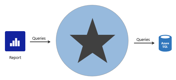
43. Each Power BI model table (except calculated tables) has a storage mode property. The storage mode property can be either Import, DirectQuery, or Dual, and it determines whether table data is stored in the model.

• Import – Queries retrieve data that’s stored, or cached, in the model.
• DirectQuery – Queries pass through to the data source.
• Dual – Queries retrieve stored data or pass through to the data source. Power BI determines the most efficient plan, striving to use cached data whenever possible.

44. Model Framework –

• An import model comprises tables that have their storage mode property set to Import.
• A DirectQuery model comprises tables that have their storage mode property set to DirectQuery, and they belong to the same source group.
• A composite model comprises more than one source group.

45. Import models are the most frequently developed model framework because there are many benefits. Import models:

• Support all Power BI data source types, including databases, files, feeds, web pages, dataflows, and more.
• Can integrate source data. For example, one table sources its data from a relational database while a related table sources its data from a web page.
• Support all DAX and Power Query (M) functionality.
• Support calculated tables.
• Deliver the best query performance. That’s because the data cached in the model is optimized for analytic queries (filter, group, and summarize) and the model is stored entirely in memory.

46. In short, import models offer you the most options and design flexibility, and they deliver fast performance. For this reason, Power BI Desktop defaults to use import storage mode when you “Get data.”

47. Limitations of Import Model – Power BI imposes dataset size restrictions, which limit the size of a model. When you publish the model to a shared capacity, there’s a 1-GB limit per dataset. When this size limit is exceeded, the dataset will fail to refresh. When you publish the model to a dedicated capacity (also known as Premium capacities), it can grow beyond 10-GB, providing you enable the Large dataset storage format setting for the capacity.

48. Data reduction techniques –

• Remove unnecessary columns
• Remove unnecessary rows
• Group by and summarize to raise the grain of fact tables
• Optimize column data types with a preference for numeric data
• Preference for custom columns in Power Query instead of calculated columns in the model
• Disable Power Query query load
• Disable auto date/time
• Use DirectQuery table storage, as described in later units of this module.

49. The 1-GB per dataset limit refers to the compressed size of the Power BI model, not the volume of data being collected from the source system.

50. Imported data must be periodically refreshed. Dataset data is only as current as the last successful data refresh. To keep data current, you set up scheduled data refresh, or report consumers can perform an on-demand refresh.

51. Power BI imposes limits on how often scheduled refresh operations can occur. It’s up to eight times per day in a shared capacity, and up to 48 times per day in a dedicated capacity.

52. When scheduled refresh limits aren’t acceptable, consider using DirectQuery storage tables, or creating a hybrid table. Or take a different approach, and create a real-time dataset instead.

53. By default, to refresh a table, Power BI removes all data and reloads it again. These operations can place an unacceptable burden on source systems, especially for large fact tables. To reduce this burden, you can set up the incremental refresh feature.

54. Incremental refresh automates the creation and management of time-period partitions, and intelligently update only those partitions that require refresh.

55. When your data source supports incremental refresh, it can result in faster and more reliable refreshes and reduced resource consumption of Power BI and source systems.

56. An import model and a DirectQuery model only comprise a single source group. When there’s more than one source group, the model framework is known as a composite model.

57. When the source data changes rapidly and users need to see current data, a DirectQuery model can deliver near real-time query results. Model large or fast-changing data sources use Direct query as the source group.

58. DirectQuery is also useful when the source database enforces row-level security (RLS). Instead of replicating RLS rules in your Power BI model, the source data base can enforce its rules. This approach works only for some relational databases, and it involves setting up single sign-on for the dataset data source. 

59. If your organization has security policies that restrict data leaving their premises, then it isn’t possible to import data.

A DirectQuery model that connects to an on-premises data source may be appropriate.

(You can also consider installing Power BI Report Server for on-premises reporting.)

60. analytic query vs Native Query – Typically, DirectQuery mode supports relational database sources. That’s because Power BI must translate analytic queries to native queries understood by the data source.

61. Limitations of Direct Query –

• Not all data sources are supported. Typically, only major relational database systems are supported. Power BI datasets and Azure Analysis Services models are supported too.
• All Power Query (M) transformations are not possible, because these queries must translate to native queries that are understood by source systems. So, for example, it’s not possible to use pivot or unpivot transformations.
• Analytic query performance can be slow, especially if source systems aren’t optimized (with indexes or materialized views), or there are insufficient resources for the analytic workload.
• Analytic queries can impact on source system performance. It could result in a slower experience for all workloads, including OLTP operations.

62. A composite model comprises more than one source group. Typically, there’s always the import source group and a DirectQuery source group.

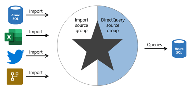
63. enterprise models benefit from using DirectQuery tables on large data sources and by boosting query performance with imported tables. Power BI features that support this scenario are described later in this unit.

64. Composite models can also boost the performance of a DirectQuery model by providing Power BI with opportunity to satisfy some analytic queries from imported data. Querying cached data almost always performs better than pass-through queries.

65. There are several limitations related to composite models.

• Import (or dual, as described later) storage mode tables still require periodic refresh. Imported data can become out of sync with DirectQuery sourced data, so it’s important to refresh it periodically.
• When an analytic query must combine imported and DirectQuery data, Power BI must consolidate source group query results, which can impact performance. To help avoid this situation for higher-grain queries, you can add import aggregation tables to your model (or enable automatic aggregations) and set related dimension tables to use dual storage mode.
• When chaining models (DirectQuery to Power BI datasets), modifications made to upstream models can break downstream models. Be sure to assess the impact of modifications by performing dataset impact analysis first.
• Relationships between tables from different source groups are known as limited relationships. A model relationship is limited when the Power BI can’t determine a “one” side of a relationship. Limited relationships may result in different evaluations of model queries and calculations.

66. SOLUTION – You can add import storage mode user-defined aggregation tables or enable automatic aggregations. This way, Power BI directs higher-grain fact queries to a cached aggregation.

To boost query performance further, ensure that related dimension tables are set to use dual storage mode. Automatic aggregations are a Premium feature.

67. A dual storage mode table is set to use both import and DirectQuery storage modes. At query time, Power BI determines the most efficient mode to use. Whenever possible, Power BI attempts to satisfy analytic queries by using cached data.

68. Slicer visuals and filter card lists, which are often based on dimension table columns, render more quickly because they’re queried from cached data.

69. iNCREMENTAL REFRESH SETTINGS –

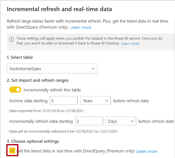
70. Configuring incremental refresh includes creating RangeStart and RangeEnd parameters, applying filters, and defining an incremental refresh policy.

Step 1 – Create parametres range start and range end with dates.

Step 2 – In Filter Rows, to specify the first condition, select is after or is after or equal to, then choose Parameter, and then choose RangeStart.

Step 3 -On the Home ribbon in Power Query Editor, select Close & Apply. 

Step 4 – Power Query loads only data specified between the RangeStart and RangeEnd parameters

step 5 – After you’ve defined RangeStart and RangeEnd parameters, and filtered data based on those parameters, you’ll define an incremental refresh policy

Step 6 – To specify the second condition, if you selected is after in the first condition, then choose is before or equal to, or if you selected is after or equal to in the first condition, then choose is before for the second condition, then choose Parameter, and then choose RangeEnd.

71. Choose the composite model framework to:

• Boost the query performance of a DirectQuery model.
• Deliver near real-time query results from an import model.
• Extend a Power BI dataset (or AAS model) with additional data.

72. When using import aggregation tables, be sure to set related dimension tables to use dual storage mode. That way, Power BI can satisfy higher-grain queries entirely from cache.

73. Plan carefully. In Power BI Desktop, it’s always possible to convert a DirectQuery table to an import table. But it’s not possible to convert an import table to a DirectQuery table.

74. Mousef is a business analyst at Adventure Works who wants to create a new model by extending the sales dataset, which is delivered by IT. Mousef wants to add a new table of census population data sourced from a web page. Which model framework should Mousef use? – A composite model would comprise a DirectQuery source group containing the sales dataset tables, and an import source group containing the imported web page data.

75. An aggregation table supports fast higher-grain queries.

76.  A hybrid table includes a DirectQuery partition for the current period to deliver near-real time results.

77. A good semantic model offers the following benefits:

• Data exploration is faster.
• Aggregations are simpler to build.
• Reports are more accurate.
• Writing reports takes less time.
• Reports are easier to maintain in the future.

78. Dimension tables contain the details about the data in fact tables: products, locations, employees, and order types. These tables are connected to the fact table through key columns.

• Dimension tables are used to filter and group the data in fact tables. The fact tables, on the other hand, contain the measurable data, such as sales and revenue, and each row represents a unique combination of values from the dimension tables.
• For the total sales orders visual, you could group the data so that you see total sales orders by product, in which product is data in the dimension table.
• Fact tables are much larger than dimension tables because numerous events occur in fact tables, such as individual sales.
• Dimension tables are typically smaller because you are limited to the number of items that you can filter and group on.
• For instance, a year contains only so many months, and the United States are composed of only a certain number of states.

79. A simple table structure will:

• Be simple to navigate because of column and table properties that are specific and user-friendly.
• Have merged or appended tables to simplify the tables within your data structure.
• Have good-quality relationships between tables that make sense.

80. Under the General tab, you can:

• Edit the name and description of the column.
• Add synonyms that can be used to identify the column when you are using the Q&A feature.
• Add a column into a folder to further organize the table structure.
• Hide or show the column.

Under the Formatting tab, you can:

• Change the data type.
• Format the date.
• Under the Advanced tab, you can:
• Sort by a specific column.
• Assign a specific category to the data.
• Summarize the data.
• Determine if the column or table contains null values.

81. Ways that you can build a common date table are:

• Source data – We recommend that you use a source date table because it is likely shared with other tools that you might be using in addition to Power BI.
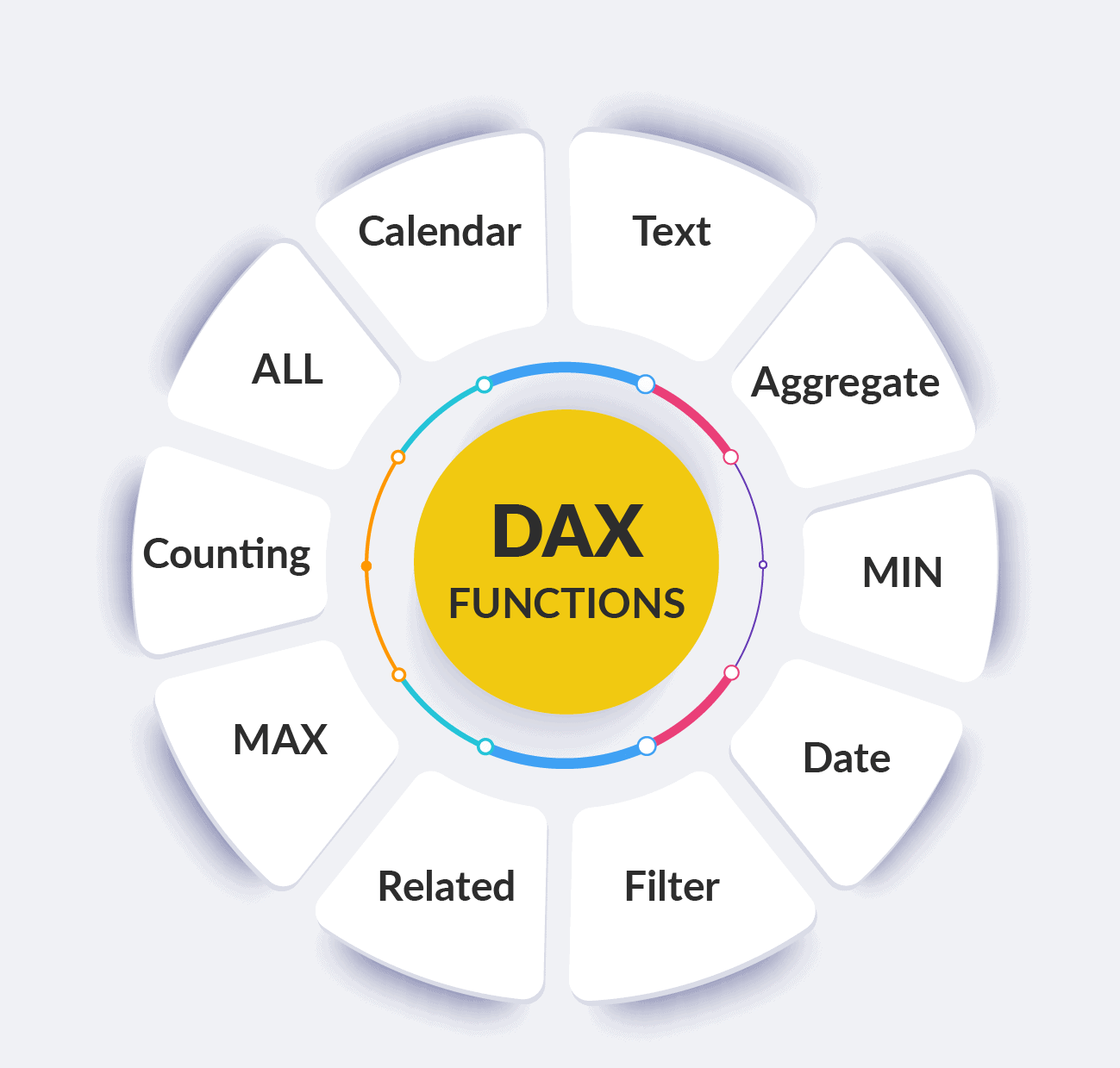
• DAX – You can use the Data Analysis Expression (DAX) functions CALENDARAUTO() or CALENDAR() to build your common date table.
  • The CALENDAR() function returns a contiguous range of dates based on a start and end date that are entered as arguments in the function.
  • Alternatively, the CALENDARAUTO() function returns a contiguous, complete range of dates that are automatically determined from your semantic model. The starting date is chosen as the earliest date that exists in your semantic model, and the ending date is the latest date that exists in your semantic model plus data that has been populated to the fiscal month that you can choose to include as an argument in the CALENDARAUTO() function. 
• Power Query – You can use M-language, the development language that is used to build queries in Power Query, to define a common date table.
  • After you have realized success in the process, you notice that you have a list of dates instead of a table of dates. To correct this error, go to the Transform tab on the ribbon and select Convert > To Table. As the name suggests, this feature will convert your list into a table. You can also rename the column to DateCol.

82. Selecting Mark as date table will remove autogenerated hierarchies from the Date field in the table that you marked as a date table. For other date fields, the auto hierarchy will still be present until you establish a relationship between that field and the date table or until you turn off the Auto Date/Time feature. You can manually add a hierarchy to your common date table by right-clicking the year, month, week, or day columns in the Fields pane and then selecting New hierarchy. This process is further discussed later in this module.

83. To determine the total sales, you need to add all sales because the Amount column in the Sales table only looks at the revenue for each sale, not the total sales revenue.

#Total Sales = SUM(Sales[‘Amount’])

84. When you are building visuals, Power BI automatically enters values of the date type as a hierarchy (if the table has not been marked as a date table).

85. Parent-child hierarchy – The Manager column determines the hierarchy and is therefore the parent, while the “children” are the employees.

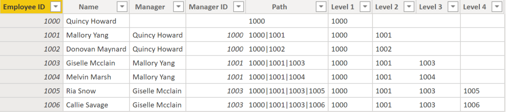
86. The process of viewing multiple child levels based on a top-level parent is known as flattening the hierarchy

87. When building a star schema, you will have dimension and fact tables. Fact tables contain information about events such as sales orders, shipping dates, resellers, and suppliers. Dimension tables store details about business entities, such as products or time, and are connected back to fact tables through a relationship.

88.  You will use PATH(), a simple DAX function that returns a text version of the managerial path for each employee, and PATHITEM() to separate this path into each level of managerial hierarchy.

89. Step 1 – While on the table, go to the Modeling tab and select New Column. In the resulting formula bar, enter the following function, which creates the text path between the employee and manager. This action creates a calculated column in DAX.

Step 2 – Path = PATH(Employee[Employee ID], Employee[Manager ID])

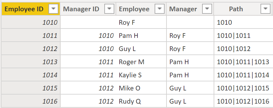
Step 3- If you look at Roger M, the path of IDs is 1010 | 1011 | 1013, which means that one level above Roger M (ID 1013) is his manager, Pam H (ID 1011), and one level above Pam H is her manager Roy F (ID 1010). In this row, Roger M is on the bottom of the hierarchy, at the child level, and Roy F is at the top of the hierarchy and is at the parent level. This path is created for every employee. To flatten the hierarchy, you can separate each level by using the PATHITEM function.

Step 4- You will use the PATHITEM function to retrieve the value that resides in the corresponding level of your hierarchy.

• Level 1 = PATHITEM(Employee[Path],1)
• Level 2 = PATHITEM(Employee[Path],2)
• Level 3 = PATHITEM(Employee[Path],3)

Step 5 – Now, you can create a hierarchy on the Fields pane, as you did previously. Right-click Level 1, because this is the first hierarchy level, and then select New Hierarchy. Then, drag and drop Level 2 and Level 3 into this hierarchy.

90. Working with role-playing dimensions requires complex DAX functions

91. The preceding visual shows the Calendar, Sales, and Order tables. Calendar is the dimension table, while Sales and Order are fact tables. The dimension table has two relationships: one with Sales and one with Order. This example is of a role-playing dimension because the Calendar table can be used to group data in both Sales and Order. If you wanted to build a visual in which the Calendar table references the Order and the Sales tables, the Calendar table would act as a role-playing dimension.

92. Data granularity is the detail that is represented within your data, meaning that the more granularity your data has, the greater the level of detail within your data.

93. Many-to-one (*:1) or one-to-many (1: *) relationship

• Describes a relationship in which you have many instances of a value in one column that are related to only one unique corresponding instance in another column.
• Describes the directionality between fact and dimension tables.
• Is the most common type of directionality and is the Power BI default when you are automatically creating relationships.
• An example of a one-to-many relationship would be between the CountryName and Territory tables, where you can have many territories that are associated with one unique country.

94. One-to-one (1:1) relationship:

• Describes a relationship in which only one instance of a value is common between two tables.
• Requires unique values in both tables.
• Is not recommended because this relationship stores redundant information and suggests that the model is not designed correctly. It is better practice to combine the tables.
• An example of a one-to-one relationship would be if you had products and product IDs in two different tables. Creating a one-to-one relationship is redundant and these two tables should be combined.

95. Many-to-many (.) relationship:

• Describes a relationship where many values are in common between two tables.
• Does not require unique values in either table in a relationship.
• Is not recommended; a lack of unique values introduces ambiguity and your users might not know which column of values is referring to what.
• For instance, the following figure shows a many-to-many relationship between the Sales and Order tables on the OrderDate column because multiple sales can have multiple orders associated with them. Ambiguity is introduced because both tables can have the same order date.

96. Data can be filtered on one or both sides of a relationship.

97. With a single cross-filter direction:

• Only one table in a relationship can be used to filter the data. For instance, Table 1 can be filtered by Table 2, but Table 2 cannot be filtered by Table 1.
• For a one-to-many or many-to-one relationship, the cross-filter direction will be from the “one” side, meaning that the filtering will occur in the table that has many values.

98. With both cross-filter directions or bi-directional cross-filtering:

• One table in a relationship can be used to filter the other. For instance, a dimension table can be filtered through the fact table, and the fact tables can be filtered through the dimension table.
• You might have lower performance when using bi-directional cross-filtering with many-to-many relationships.
• You should not enable bi-directional cross-filtering relationships unless you fully understand the ramifications of doing so. Enabling it can lead to ambiguity, over-sampling, unexpected results, and potential performance degradation.

99. For one-to-one relationships, the only option that is available is bi-directional cross-filtering. Data can be filtered on either side of this relationship and result in one distinct, unambiguous value. For instance, you can filter on one Product ID and be returned a single Product, and you can filter on a Product and be returned a single Product ID.

100. For many-to-many relationships, you can choose to filter in a single direction or in both directions 

101. The ambiguity that is associated with bi-directional cross-filtering is amplified in a many-to-many relationship because multiple paths will exist between different tables

102. many-to-many relationships and/or bi-directional relationships are complicated. Unless you are certain what your data looks like when aggregated, these types of open-ended relationships with multiple filtering directions can introduce multiple paths through the data.

103. Consider the scenario where you are tasked with building a visual that examines budgets for customers and accounts. You can have multiple customers on the same account and multiple accounts with the same customer, so you know that you need to create a many-to-many relationship.

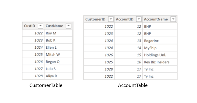
104. To create this relationship, go to Manage Relationships > New. In the resulting window, create a relationship between the Customer ID column in CustomerTable and AccountTable.

The relationship is set to many-to-many, and the filter type is in both directions. Immediately, you will be warned that you should only use this type of relationship if it is expected that neither column will have unique values because you might get unexpected values.

Because you want to filter in both directions, choose bi-directional cross-filtering.

105. Fact tables contain observational data such as sales orders, employees, shipping dates, and so on, while dimension tables contain information about specific entities such as product IDs and dates.

106. Cardinality is the measure of unique values in a table. An example of high cardinality would be a Sales table as it has a high number of unique values.

107. You can write a DAX formula to add a calculated table to your model. The formula can duplicate or transform existing model data, or create a series of data, to produce a new table

108. Calculated table data is always imported into your model, so it increases the model storage size and can prolong data refresh time.

109. A calculated table can’t connect to external data; you need to use Power Query to accomplish that task.

110. Calculated tables can be useful in various scenarios:

• Date tables
• Role-playing dimensions
• What-if analysis

111. Date tables are required to apply special time filters known as time intelligence. DAX time intelligence functions only work correctly when a date table is set up. When your source data doesn’t include a date table, you can create one as calculated tables by using the CALENDAR or CALENDARAUTO DAX functions.

112. When two model tables have multiple relationships, it could be because your model has a role-playing dimension. For example, if you have a table named Sales that includes two date columns, OrderDateKey and ShipDateKey, both columns are related to the Date column in the Date table. In this case, the Date table is described as a role-playing dimension because it could play the role of order date or ship date.

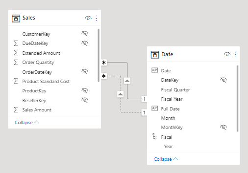
113. Microsoft Power BI models only allow one active relationship between tables, which in the model diagram is indicated as a solid line. The active relationship is used by default to propagate filters, which in this case would be from the Date table to the OrderDateKey column in the Sales table.

114.

Any remaining relationships between the two tables are inactive. In a model diagram, the relationships are represented as dashed lines. Inactive relationships are only used when they’re expressly requested in a calculated formula by using the USERELATIONSHIP DAX function.

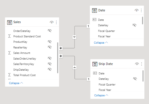
115. Perhaps a better model design could have two date tables, each with an active relationship to the Sales table. Thus, report users can filter by order date or ship date, or both at the same time. A calculated table can duplicate the Date table data to create the Ship Date table.

116. Power BI Desktop supports a feature called What-if parameters. When you create a what-if parameter, a calculated table is automatically added to your model.

117.  write a DAX formula to add a calculated column to any table in your model. The formula is evaluated for each table row and it returns a single value

118. When added to an Import storage mode table, the formula is evaluated when the semantic model is refreshed, and it increases the storage size of your model. When added to a DirectQuery storage mode table, the formula is evaluated by the underlying source database when the table is queried.

119. write a DAX formula to add a measure to any table in your model. The formula is concerned with achieving summarization over model data. Similar to a calculated column, the formula must return a single value.

120. Unlike calculated columns, which are evaluated at data refresh time, measures are evaluated at query time. Their results are never stored in the model.

121. In the Fields pane, measures are shown with the calculator icon. 

122. explicit measures are model calculations that are written in DAX and are commonly referred to as simply measures. Yet, the concept of implicit measures exists, too.

123. Implicit measures are columns that can be summarized by visuals in simplistic ways, like count, sum, minimum, maximum, and so on. You can identify implicit measures in the Fields pane because they’re shown with the sigma symbol ( ∑ ).

124. Any column can be summarized when added to a visual. Therefore, whether they’re shown with the sigma symbol or not, when they’re added to a visual, they can be set up as implicit measures.

125. no such concept as a calculated measure exists in tabular modeling. The word calculated is used to describe calculated tables and calculated columns, which distinguishes them from tables and columns that originate from Power Query. Power Query doesn’t have the concept of an explicit measure.

126. A DAX formula consists of expressions that return a result. The result is either a table object or a scalar value. Calculated table formulas must return a table object; calculated column and measure formulas must return a scalar value (single value).

127.  IntelliSense is a code-completion aid that lists functions and model resources. When you select a DAX function, it also provides you with a definition and description. We recommend that you use IntelliSense to help you quickly build accurate formulas.

128. DAX is a functional language meaning that formulas rely on functions to accomplish specific goals. Typically, DAX functions have arguments that allow passing in variables. Formulas can use many function calls and will often nest functions within other functions.

129. Formulas can only refer to three types of model objects: tables, columns, or measures. A formula can’t refer to a hierarchy or a hierarchy level. (Recall that a hierarchy level is based on a column, so your formula can refer to a hierarchy level’s column.)

130. When you reference a table in a formula, officially, the table name is enclosed within single quotation marks. In the following calculated table definition, notice that the Date table is enclosed within single quotation marks.

Ship Date = ‘Date’

131. single quotation marks can be omitted when both of the following conditions are true:

1. The table name does not include embedded spaces.
2. The table name isn’t a reserved word that’s used by DAX. All DAX function names and operators are reserved words. Date is a DAX function name, which explains why, when you are referencing a table named Date, that you must enclose it within single quotation marks.

132. In the following calculated table definition, it’s possible to omit the single quotation marks when referencing the Airport table:          Arrival Airport = Airport

133. When you reference a column in a formula, the column name must be enclosed within square brackets. Optionally, it can be preceded by its table name. For example, the following measure definition refers to the Sales Amount column.

134. Because column names are unique within a table but not necessarily unique within the model, you can disambiguate the column reference by preceding it with its table name. This disambiguated column is known as a fully qualified column. Some DAX functions require passing in fully qualified columns.

Revenue = SUM(Sales[Sales Amount])

Revenue = SUM([Sales Amount])

135. When you reference a measure in a formula, like column name references, the measure name must be enclosed within square brackets. For example, the following measure definition refers to the Revenue and Cost measures.

Profit = [Revenue] – [Cost]

136. It’s possible to precede a measure reference with its table name. However, measures are a model-level object. While they’re assigned to a home table, it’s only a cosmetic relationship to logically organize measures in the Fields pane.

Therefore, while we recommend that you always precede a column reference with its table name, the inverse is true for measures: We recommend that you never precede a measure reference with its table name.

137. Whitespace refers to characters that you can use to format your formulas in a way that’s quick and simple to understand. Whitespace characters include:

• Spaces
• Tabs
• Carriage returns

138. Whitespace is optional and it doesn’t modify your formula logic or negatively impact performance. We strongly recommend that you adopt a format style and apply it consistently, and consider the following recommendations:

• Use spaces between operators.
• Use tabs to indent nested function calls.
• Use carriage returns to separate function arguments, especially when it’s too long to fit on a single line. Formatting in this way makes it simpler to troubleshoot, especially when the formula is missing a parenthesis.
• Err on the side of too much whitespace than too little.

139. In the formula bar, to enter a carriage return, press Shift+Enter. Pressing Enter alone will commit your formula.

140.

Revenue YoY % =
DIVIDE(
[Revenue]
– CALCULATE(
[Revenue],
SAMEPERIODLASTYEAR(‘Date'[Date])
),
CALCULATE(
[Revenue],
SAMEPERIODLASTYEAR(‘Date'[Date])
)
)

140. An excellent formatting tool from another source that can help you format your calculations is DAX Formatter. This tool allows you to paste in your calculation and format it. You can then copy the formatted calculation to the clipboard and paste it back into Power BI Desktop.

141. The BLANK data type deserves a special mention. DAX uses BLANK for both database NULL and for blank cells in Excel. BLANK doesn’t mean zero. Perhaps it might be simpler to think of it as the absence of a value.

142. Two DAX functions are related to the BLANK data type: the BLANK DAX function returns BLANK, while the ISBLANK DAX function tests whether an expression evaluates to BLANK.

143. Many functions exist that you won’t find in Excel because they’re specific to data modeling:

• Relationship navigation functions
• Filter context modification functions
• Iterator functions
• Time intelligence functions
• Path functions

144. The IF DAX function tests whether a condition that’s provided as the first argument is met. It returns one value if the condition is TRUE and returns the other value if the condition is FALSE

145. Many Excel summarization functions are available, including SUM, COUNT, AVERAGE, MIN, MAX, and many others. The only difference is that in DAX, you pass in a column reference, whereas in Excel, you pass in a range of cells.

146. Many Excel mathematic, text, date and time, information, and logical functions are available as well. For example, a small sample of Excel functions that are available in DAX include ABS, ROUND, SQRT, LEN, LEFT, RIGHT, UPPER, DATE, YEAR, MONTH, NOW, ISNUMBER, TRUE, FALSE, AND, OR, NOT, and IFERROR

147. Two useful DAX functions that aren’t specific to modeling and that don’t originate from Excel are DISTINCTCOUNT and DIVIDE.

148. You can use the DISTINCTCOUNT DAX function to count the number of distinct values in a column. This function is especially powerful in an analytics solution.

149. Consider that the count of customers is different from the count of distinct customers. The latter doesn’t count repeat customers, so the difference is “How many customers” compared with “How many different customers.”

150. You can use the DIVIDE DAX function to achieve division. You must pass in numerator and denominator expressions. Optionally, you can pass in a value that represents an alternate result

DIVIDE(<numerator>, <denominator>[, <alternate_result>])

151. The DIVIDE function automatically handles division by zero cases. If an alternate result isn’t passed in, and the denominator is zero or BLANK, the function returns BLANK.

152. We recommend that you use the DIVIDE function whenever the denominator is an expression that could return zero or BLANK. In the case that the denominator is a constant value, we recommend that you use the divide operator (/), which is introduced later in this module. In this case, the division is guaranteed to succeed, and your expression will perform better because it will avoid unnecessary testing.

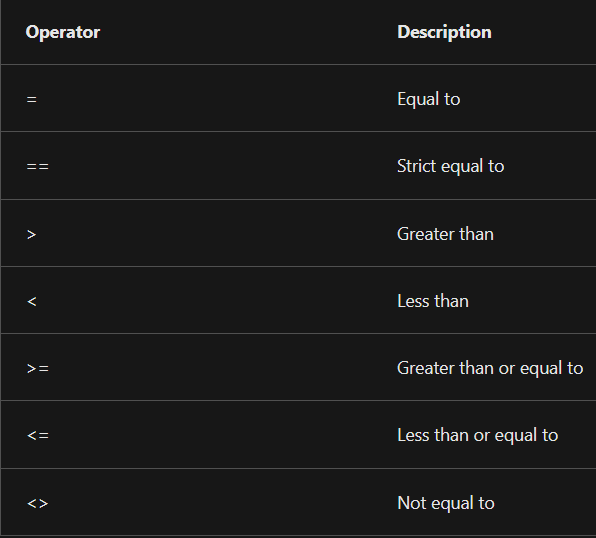
153. Comparison operators

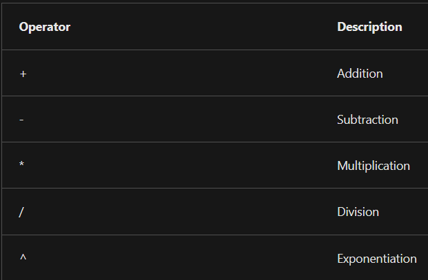
154. Arithmetic operators

155. Text concatenation operator – Use the ampersand (&) character to connect, or concatenate, two text values to produce one continuous text value. 

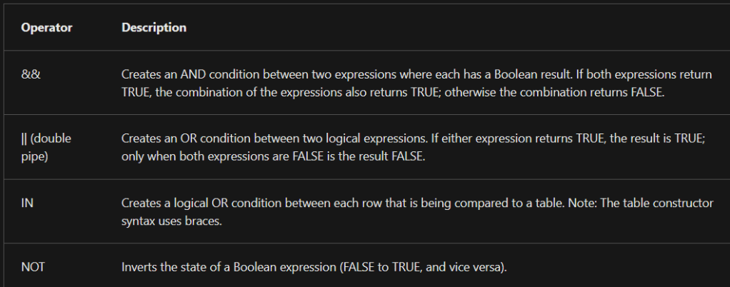
156. Logical operators – Use logical operators to combine expressions that produce a single result. 

157. An example that uses the IN logical operator is the ANZ Revenue measure definition, which uses the CALCULATE DAX function to enforce a specific filter of two countries: Australia and New Zealand.

158. ANZ Revenue = CALCULATE( [Revenue], Customer[Country-Region] IN { “Australia”, “New Zealand” } )

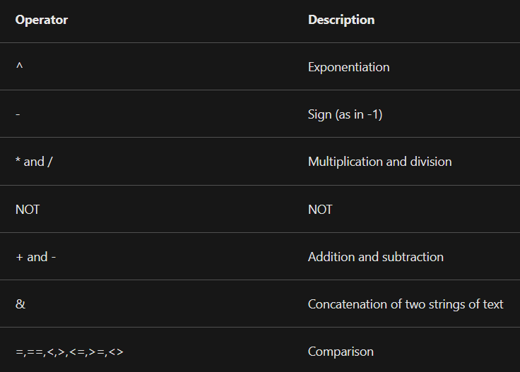
159. Operator precedence – When your DAX formula includes multiple operators, DAX uses rules to determine the evaluation order, which is known as an operator precedence.

160. We recommend that you use variables because they offer several benefits:

1. Improve performance
2. Improve readability
3. Simplify debugging
4. Reduce complexity

• Improving the readability and maintenance of your formulas.
• Improving performance because variables are evaluated once and only when or if they’re needed.
• Allowing (at design time) straightforward testing of a complex formula by returning the variable of interest.

161. Notice that the RETURN clause refers to the variable twice. This improved measure definition formula will run in at least half the time because it doesn’t need to evaluate the prior year’s revenue twice.

Sample variable example below.

Revenue YoY % =
VAR RevenuePriorYear =
CALCULATE(
[Revenue],
SAMEPERIODLASTYEAR(‘Date'[Date])
)
RETURN
DIVIDE(
[Revenue] – RevenuePriorYear,
RevenuePriorYear
)

162. You’re using Power BI Desktop to develop a model. It has a table named Geography, which has two relationships to the Sales table. One relationship filters by customer region and the other filters by sales region. You need to create a role-playing dimension so that both filters are possible. What type of DAX calculation will you add to the model?

A calculated table could create a table that duplicates the Geography table data. It could then have an active relationship to the Sales table. Both geography tables would have active relationships to allow report users to filter by customer region or sales region.

163. You write a DAX formula that adds BLANK to the number 20. What will be the result? The result will be 20 – BLANK is converted to zero when added to a number.

164. Measures in Microsoft Power BI models are either implicit or explicit. Implicit measures are automatic behaviors that allow visuals to summarize model column data. Explicit measures, also known simply as measures, are calculations that you can add to your model. This module focuses on how you can use implicit measures

165. Numeric columns support the greatest range of aggregation functions:

• Sum
• Average
• Minimum
• Maximum
• Count (Distinct)
• Count
• Standard deviation
• Variance
• Median

166. The default summarization is now set to Average (the modeler knows that it’s inappropriate to sum unit price values together because they’re rates, which are non-additive).

167. Non-numeric columns can be summarized. However, the sigma symbol does not show next to non-numeric columns in the Fields pane because they don’t summarize by default.

Text columns allow the following aggregations:

• First (alphabetically)
• Last (alphabetically)
• Count (Distinct)
• Count

Date columns allow the following aggregations:

• Earliest
• Latest
• Count (Distinct)
• Count

Boolean columns allow the following aggregations:

• Count (Distinct)
• Count

168. Several benefits are associated with implicit measures.

• Implicit measures are simple concepts to learn and use, and
• They provide flexibility in the way that report authors visualize model data.
• Additionally, they mean less work for you as a data modeler because you don’t have to create explicit calculations.

169. Implicit measures don’t work when the model is queried by using Multidimensional Expressions (MDX)

170. Immediately after you create a measure, set the formatting options to ensure well-presented and consistent values in all report visuals.

171. The COUNT DAX function counts the number of non-BLANK values in a column, while the DISTINCTCOUNT DAX function counts the number of distinct values in a column. Because an order can have one or more order lines, the Sales Order column will have duplicate values. A distinct count of values in this column will correctly count the number of orders.

172. you can choose the better way to write the Order Line Count measure. Instead of counting values in a column, it’s semantically clearer to use the COUNTROWS DAX function.

Order Line Count =
COUNT(Sales[SalesOrderLineKey])

Order Count =
DISTINCTCOUNT(‘Sales Order'[Sales Order])

Order Line Count =
COUNTROWS(Sales)

173. All measures that you’ve created are considered simple measures because they aggregate a single column or single table.

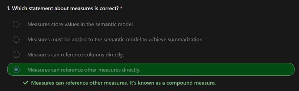
174. When a measure references one or more measures, it’s known as a compound measure.

Profit =
[Revenue] – [Cost]

175. Now that your model provides a way to summarize profit, you can delete the Profit Amount calculated column.

By removing this calculated column, you’ve optimized the semantic model. Removing this columns results in a decreased semantic model size and shorter data refresh times. The Profit Amount calculated column wasn’t required because the Profit measure can directly produce the required result.

176. Regarding similarities between calculated columns and measures, both are:

• Calculations that you can add to your semantic model.
• Defined by using a DAX formula.
• Referenced in DAX formulas by enclosing their names within square brackets.

177. The areas where calculated columns and measures differ include:

• Purpose – Calculated columns extend a table with a new column, while measures define how to summarize model data.
• Evaluation – Calculated columns are evaluated by using row context at data refresh time, while measures are evaluated by using filter context at query time. Filter context is introduced in a later module; it’s an important topic to understand and master so that you can achieve complex summarizations.
• Storage – Calculated columns (in Import storage mode tables) store a value for each row in the table, but a measure never stores values in the model.
• Visual use – Calculated columns (like any column) can be used to filter, group, or summarize (as an implicit measure), whereas measures are designed to summarize.

178.

179.

180. Calculated tables have a cost: They increase the model storage size and they can prolong the data refresh time. The reason is because calculated tables recalculate when they have formula dependencies to refreshed tables.

181. In the model diagram, notice that the Sales table has three relationships to the Date table.

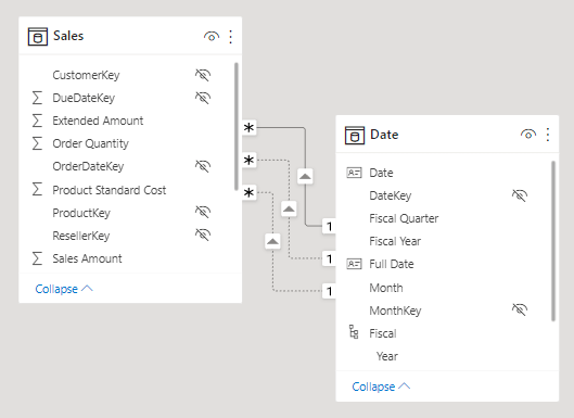
The calculated table definition duplicates the Date table data to produce a new table named Ship Date. The Ship Date table has exactly the same columns and rows as the Date table. When the Date table data refreshes, the Ship Date table recalculates, so they’ll always be in sync.

It’s possible to rename columns of a calculated table. In this example, it’s a good idea to rename columns so that they better describe their purpose. For example, the Fiscal Year column in the Ship Date table can be renamed as Ship Fiscal Year. Accordingly, when fields from the Ship Date table are used in visuals, their names are automatically included in captions like the visual title or axis labels.

182. calculated tables are useful to work in scenarios when multiple relationships between two tables exist, as previously described.

They can also be used to add a date table to your model. Date tables are required to apply special time filters known as time intelligence.

183. The CALENDARAUTO DAX function takes a single optional argument, which is the last month number of the year, and returns a single-column table. If you don’t pass in a month number, it’s assumed to be 12 (for December). For example, at Adventure Works, their financial year ends on June 30 of each year, so the value 6 (for June) is passed in.

184. The CALENDARAUTO function guarantees that the following requirements to mark a date table are met:

• The table must include a column of data type Date.
• The column must contain complete years.
• The column must not have missing dates.

DateDAX = CALENDAR(DATE(2013,01,01),DATE(2016, 12, 31))

185.

Due Fiscal Year =
“FY”
& YEAR(‘Due Date'[Due Date])
+ IF(
MONTH(‘Due Date'[Due Date]) > 6,
1
)

186.

Due Fiscal Quarter =
‘Due Date'[Due Fiscal Year] & ” Q”
& IF(
MONTH(‘Due Date'[Due Date]) <= 3,
3,
IF(
MONTH(‘Due Date'[Due Date]) <= 6,
4,
IF(
MONTH(‘Due Date'[Due Date]) <= 9,
1,
2
)
)
)

187.

Due Month =
FORMAT(‘Due Date'[Due Date], “yyyy mmm”)

188.

Due Full Date =
FORMAT(‘Due Date'[Due Date], “yyyy mmm, dd”)

189.

MonthKey =
(YEAR(‘Due Date'[Due Date]) * 100) + MONTH(‘Due Date'[Due Date])

190. Row context –

Due Fiscal Year =
“FY”
& YEAR(‘Due Date'[Due Date])
+ IF(
MONTH(‘Due Date'[Due Date]) <= 6,
1
)

190. Row context doesn’t extend beyond the table. If your formula needs to reference columns in other tables, you have two options:

• If the tables are related, directly or indirectly, you can use the RELATED or RELATEDTABLE DAX function. The RELATED function retrieves the value at the one-side of the relationship, while the RELATEDTABLE retrieves values on the many-side. The RELATEDTABLE function returns a table object.
• When the tables aren’t related, you can use the LOOKUPVALUE DAX function.

191. Generally, try to use the RELATED function whenever possible. It will usually perform better than the LOOKUPVALUE function due to the ways that relationship and column data is stored and indexed.

192.

Discount Amount =
(
Sales[Order Quantity]
* RELATED(‘Product'[List Price])
) – Sales[Sales Amount]

193. The calculated column definition adds the Discount Amount column to the Sales table. Power BI evaluates the calculated column formula for each row of the Sales table. The values for the Order Quantity and Sales Amount columns are retrieved within row context. However, because the List Price column belongs to the Product table, the RELATED function is required to retrieve the list price value for the sale product.

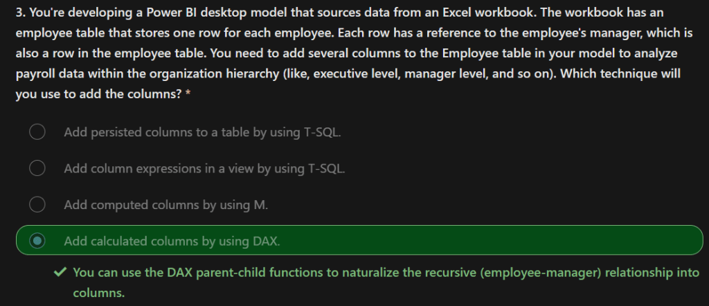
194. There are three techniques that you can use to add columns to a model table:

• Add columns to a view or table (as a persisted column), and then source them in Power Query. This option only makes sense when your data source is a relational database and if you have the skills and permissions to do so. However, it’s a good option because it supports ease of maintenance and allows reuse of the column logic in other models or reports.
• Add custom columns (using M) to Power Query queries.
• Add calculated columns (using DAX) to model tables.

195. When you need to add a column to a calculated table, make sure that you create a calculated column.

196. Otherwise, we recommend that you only use a calculated column when the calculated column formula:

• Depends on summarized model data.
• Needs to use specialized modeling functions that are only available in DAX, such as the RELATED and RELATEDTABLE functions.
• Specialized functions can also include the DAX parent and child hierarchies, which are designed to naturalize a recursive relationship into columns, for example, in an employee table where each row stores a reference to the row of the manager (who is also an employee).

197.

198.

199.

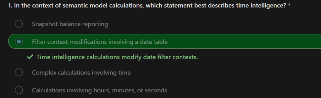
200. Time intelligence calculations modify date filter contexts. They can help you answer these time-related questions:

• What’s the accumulation of revenue for the year, quarter, or month?
• What revenue was produced for the same period last year?
• What growth in revenue has been achieved over the same period last year?
• How many new customers made their first order in each month?
• What’s the inventory stock on-hand value for the company’s products?

201. A date table is a table that meets the following requirements:

• It must have a column of data type Date (or date/time), known as the date column.
• The date column must contain unique values.
• The date column must not contain BLANKs.
• The date column must not have any missing dates.
• The date column must span full years. A year isn’t necessarily a calendar year (January-December).
• The date table must be indicated as a date table.

202. One group of DAX time intelligence functions is concerned with summarizations over time:

• DATESYTD – Returns a single-column table that contains dates for the year-to-date (YTD) in the current filter context. This group also includes the DATESMTD and DATESQTD DAX functions for month-to-date (MTD) and quarter-to-date (QTD). You can pass these functions as filters into the CALCULATE DAX function.
• TOTALYTD – Evaluates an expression for YTD in the current filter context. The equivalent QTD and MTD DAX functions of TOTALQTD and TOTALMTD are also included.
• DATESBETWEEN – Returns a table that contains a column of dates that begins with a given start date and continues until a given end date.
• DATESINPERIOD – Returns a table that contains a column of dates that begins with a given start date and continues for the specified number of intervals.

203. While the TOTALYTD function is simple to use, you are limited to passing in one filter expression. If you need to apply multiple filter expressions, use the CALCULATE function and then pass the DATESYTD function in as one of the filter expressions.

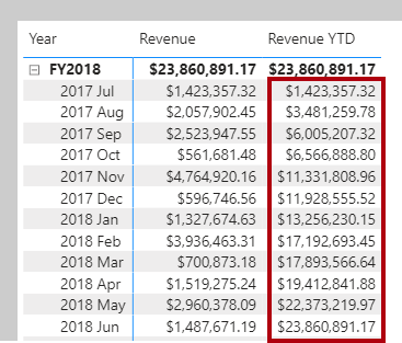
204. On Page 1 of the report, add the Revenue YTD measure to the matrix visual. Notice that it produces a summarization of the revenue amounts from the beginning of the year through to the filtered month.

Revenue YTD =
TOTALYTD([Revenue], ‘Date'[Date], “6-30”)

205. Another group of DAX time intelligence functions is concerned with shifting time periods:

• DATEADD – Returns a table that contains a column of dates, shifted either forward or backward in time by the specified number of intervals from the dates in the current filter context.
• PARALLELPERIOD – Returns a table that contains a column of dates that represents a period that is parallel to the dates in the specified dates column, in the current filter context, with the dates shifted a number of intervals either forward in time or back in time.
• SAMEPERIODLASTYEAR – Returns a table that contains a column of dates that are shifted one year back in time from the dates in the specified dates column, in the current filter context.
• Many helper DAX functions for navigating backward or forward for specific time periods, all of which returns a table of dates. These helper functions include NEXTDAY, NEXTMONTH, NEXTQUARTER, NEXTYEAR, and PREVIOUSDAY, PREVIOUSMONTH, PREVIOUSQUARTER, and PREVIOUSYEAR.

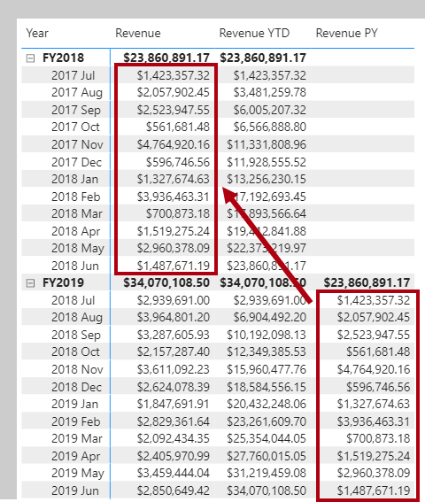
206. Add the Revenue PY measure to the matrix visual. Notice that it produces results that are similar to the previous year’s revenue amounts.

Revenue PY =
VAR RevenuePriorYear = CALCULATE([Revenue], SAMEPERIODLASTYEAR(‘Date'[Date]))
RETURN
RevenuePriorYear

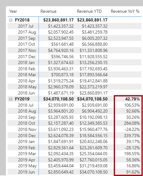
207. You will modify the measure by renaming it to Revenue YoY % and then updating the RETURN clause to calculate the change ratio. Be sure to change the format to a percentage with two decimals places.

Revenue YoY % =
VAR RevenuePriorYear = CALCULATE([Revenue], SAMEPERIODLASTYEAR(‘Date'[Date]))
RETURN
DIVIDE(
[Revenue] – RevenuePriorYear,
RevenuePriorYear
)

208. The FIRSTDATE and the LASTDATE DAX functions return the first and last date in the current filter context for the specified column of dates.

209. Life-to-date means from the beginning of time until the last date in filter context. The following example shows how you can calculate the number of new customers for a time period. A new customer is counted in the time period in which they made their first purchase.

Customers LTD =
VAR CustomersLTD =
CALCULATE(
DISTINCTCOUNT(Sales[CustomerKey]),
DATESBETWEEN(
‘Date'[Date],
BLANK(),
MAX(‘Date'[Date])
),
‘Sales Order'[Channel] = “Internet”
)
RETURN
CustomersLTD

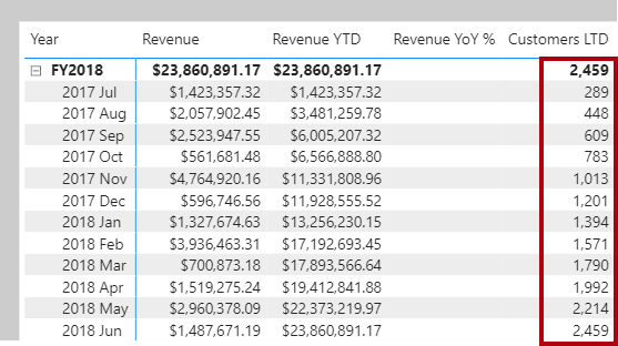
210. The DATESBETWEEN function returns a table that contains a column of dates that begins with a given start date and continues until a given end date. When the start date is BLANK, it will use the first date in the date column. (Conversely, when the end date is BLANK, it will use the last date in the date column.) 

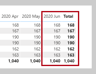
211. Snapshot calculations – When you are summarizing snapshot tables, measure formulas can rely on DAX time intelligence functions to enforce a single date filter.

212. The date will be the last date of each time period. It’s achieved by using the LASTDATE function.

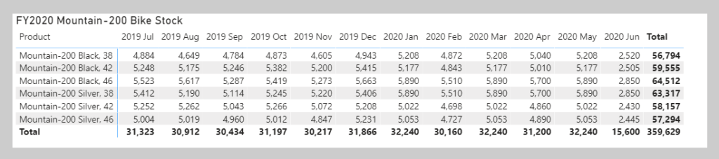
Stock on Hand =
CALCULATE(
SUM(Inventory[UnitsBalance]),
LASTDATE(‘Date'[Date])
)

213. The LASTNONBLANK function evaluates its expression in row context. The CALCULATE function must be used to transition the row context to filter context to correctly evaluate the expression.

214.

Stock on Hand =
CALCULATE(
SUM(Inventory[UnitsBalance]),
LASTNONBLANK(
‘Date'[Date],
CALCULATE(SUM(Inventory[UnitsBalance]))
)
)

215.

216.

217.

218. Performance optimization, also known as performance tuning, involves making changes to the current state of the semantic model so that it runs more efficiently. Essentially, when your semantic model is optimized, it performs better.

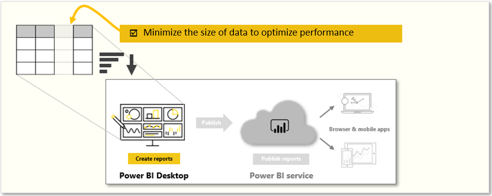
219. A smaller sized semantic model uses less resources (memory) and achieves faster data refresh, calculations, and rendering of visuals in reports. Therefore, the performance optimization process involves minimizing the size of the semantic model and making the most efficient use of the data in the model

220. Best Practices to follow for better perfromance.

• Ensuring that the correct data types are used.
• Deleting unnecessary columns and rows.
• Avoiding repeated values.
• Replacing numeric columns with measures.
• Reducing cardinalities.
• Analyzing model metadata.
• Summarizing data where possible.

221.

222. The users are happy with the results that they see in the report, but they are not satisfied with the report performance. Loading the pages in the report is taking too long, and tables are not refreshing quickly enough when certain selections are made.

223. If your semantic model has multiple tables, complex relationships, intricate calculations, multiple visuals, or redundant data, a potential exists for poor report performance. The poor performance of a report leads to a negative user experience.

224. Performance analyzer will help you identify the elements that are contributing to your performance issues, which can be useful during troubleshooting.

225. Before you run Performance analyzer, to ensure you get the most accurate results in your analysis (test), make sure that you start with a clear visual cache and a clear data engine cache.

226.

• Visual cache – When you load a visual, you can’t clear this visual cache without closing Power BI Desktop and opening it again. To avoid any caching in play, you need to start your analysis with a clean visual cache.
• To ensure that you have a clear visual cache, add a blank page to your Power BI Desktop (.pbix) file and then, with that page selected, save and close the file. Reopen the Power BI Desktop (.pbix) file that you want to analyze. It will open on the blank page.
• Data engine cache – When a query is run, the results are cached, so the results of your analysis will be misleading. You need to clear the data cache before rerunning the visual.
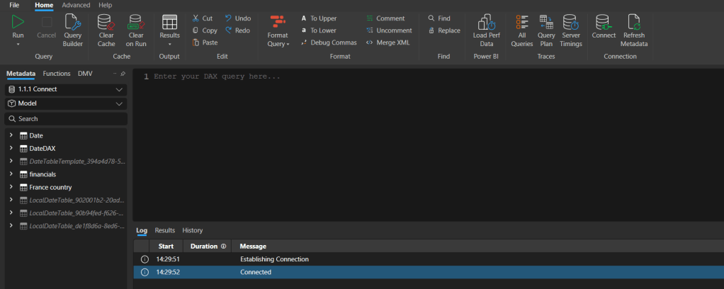
• To clear the data cache, you can either restart Power BI Desktop or connect DAX Studio to the semantic model and then call Clear Cache.

227. When you have cleared the caches and opened the Power BI Desktop file on the blank page, go to the View tab and select the Performance analyzer option.

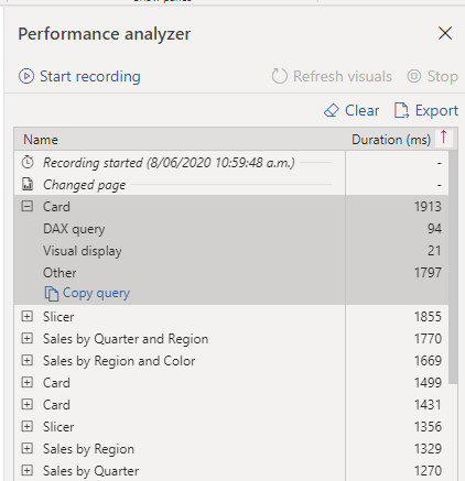
228. You can review the results of your performance test in the Performance analyzer pane. To review the tasks in order of duration, longest to shortest, right-click the Sort icon next to the Duration (ms) column header, and then select Total time in Descending order.

229. The log information for each visual shows how much time it took (duration) to complete the following categories of tasks:

• DAX query – The time it took for the visual to send the query, along with the time it took Analysis Services to return the results.
• Visual display – The time it took for the visual to render on the screen, including the time required to retrieve web images or geocoding.
• Other – The time it took the visual to prepare queries, wait for other visuals to complete, or perform other background processing tasks. If this category displays a long duration, the only real way to reduce this duration is to optimize DAX queries for other visuals, or reduce the number of visuals in the report.

230.

231. Resolve issues and optimize performance

Consider the number of visuals on the report page; fewer visuals means better performance.

other ways to provide additional details, such as drill-through pages and report page tooltips.

Examine the number of fields in each visual. Ask yourself if you really need all of this data in a visual. You might find that you can reduce the number of fields that you currently use.

The upper limit for visuals is 100 fields (measures or columns), so a visual with more than 100 fields will be slow to load.

232. A good starting point is any DAX query that is taking longer than 120 milliseconds

Count Customers =
CALCULATE (
DISTINCTCOUNT ( Order[ProductID] ),
FILTER ( Order, Order[OrderQty] >= 5 )
)

In the following example, the FILTER function was replaced with the KEEPFILTER function. When the test was run again in Performance analyzer, the duration was shorter as a result of the KEEPFILTER function.

Count Customers =
CALCULATE (
DISTINCTCOUNT ( Order[ProductID] ),
KEEPFILTERS (Order[OrderQty] >= 5 )
)

233.  if the DAX query is displaying a high duration value, it is likely that a measure is written poorly or an issue has occurred with the semantic model. The issue might be caused by the relationships, columns, or metadata in your model, or it could be the status of the Auto date/time option, as explained in the following section.

234. Check that relationship cardinality properties are correctly configured.

235. For example, a one-side column that contains unique values might be incorrectly configured as a many-side column. 

236.It is best practice to not import columns of data that you do not need.

237.To avoid deleting columns in Power Query Editor, you should try to deal with them at the source when loading data into Power BI Desktop

238.However, if it is impossible to remove redundant columns from the source query or the data has already been imported in its raw state

239. if you find that a column adds no value, you should remove it from your semantic model. For example, suppose that you have an ID column with thousands of unique rows. You know that you won’t use this particular column in a relationship, so it will not be used in a report. Therefore, you should consider this column as unnecessary and admit that it is wasting space in your semantic model.

240. Data reduction techniques for Import modeling

1. Remove unnecessary columns
2. Remove unnecessary rows
3. Group by and summarize
4. Optimize column data types
5. Preference for custom columns
6. Disable Power Query query load
7. Disable auto date/time
8. Switch to Mixed mode

241. four compelling reasons include:

• Larger model sizes may not be supported by your capacity. Shared capacity can host models up to 1 GB in size, while Premium capacities can host larger models depending on the SKU. For further information, read the Power BI Premium support for large semantic models article. (Semantic models were previously known as datasets.)
• Smaller model sizes reduce contention for capacity resources, in particular memory. It allows more models to be concurrently loaded for longer periods of time, resulting in lower eviction rates.
• Smaller models achieve faster data refresh, resulting in lower latency reporting, higher semantic model refresh throughput, and less pressure on source system and capacity resources.
• Smaller table row counts can result in faster calculation evaluations, which can deliver better overall query performance.

242. Model table columns serve two main purposes:

• Reporting, to achieve report designs that appropriate filter, group, and summarize model data
• Model structure, by supporting model relationships, model calculations, security roles, and even data color formatting

243. Columns that don’t serve these purposes can probably be removed. Removing columns is referred to as vertical filtering

244.It can be achieved by loading filtered rowsets into model tables for two different reasons: to filter by entity or by time. Removing rows is referred to as horizontal filtering

245.The Power Query options include:

• Unnecessary columns – Evaluates the need for each column. If one or more columns will not be used in the report and are therefore unnecessary, you should remove them by using the Remove Columns option on the Home tab.
• Unnecessary rows – Checks the first few rows in the semantic model to see if they are empty or if they contain data that you do not need in your reports; if so, it removes those rows by using the Remove Rows option on the Home tab.
• Data type – Evaluates the column data types to ensure that each one is correct. If you identify a data type that is incorrect, change it by selecting the column, selecting Data Type on the Transform tab, and then selecting the correct data type from the list.
• Query names – Examines the query (table) names in the Queries pane. Just like you did for column header names, you should change uncommon or unhelpful query names to names that are more obvious or names that the user is more familiar with. You can rename a query by right-clicking that query, selecting Rename, editing the name as required, and then pressing Enter.
• Column details – Power Query Editor has the following three data preview options that you can use to analyze the metadata that is associated with your columns. You can find these options on the View tab, as illustrated in the following screenshot.
  • Column quality – Determines what percentage of items in the column are valid, have errors, or are empty. If the Valid percentage is not 100, you should investigate the reason, correct the errors, and populate empty values.
  • Column distribution – Displays frequency and distribution of the values in each of the columns. You will investigate this further later in this module.
  • Column profile – Shows column statistics chart and a column distribution chart.

246. If you are reviewing a large semantic model with more than 1,000 rows, and you want to analyze that whole semantic model, you need to change the default option at the bottom of the window. Select Column profiling based on top 1000 rows > Column profiling based on entire data set.

247. Other metadata that you should consider is the information about the semantic model as a whole, such as the file size and data refresh rates. You can find this metadata in the associated Power BI Desktop (.pbix) file. The data that you load into Power BI Desktop is compressed and stored to the disk.

248. If your semantic model has multiple tables, complex relationships, intricate calculations, multiple visuals, or redundant data, a potential exists for poor report performance. The poor performance of a report leads to a negative user experience.

249. Two types of cache

• Visual cache – When you load a visual, you can’t clear this visual cache without closing Power BI Desktop and opening it again. To avoid any caching in play, you need to start your analysis with a clean visual cache.To ensure that you have a clear visual cache, add a blank page to your Power BI Desktop (.pbix) file and then, with that page selected, save and close the file. Reopen the Power BI Desktop (.pbix) file that you want to analyze. It will open on the blank page.
• Data engine cache – When a query is run, the results are cached, so the results of your analysis will be misleading. You need to clear the data cache before rerunning the visual.To clear the data cache, you can either restart Power BI Desktop or connect DAX Studio to the semantic model and then call Clear Cache.

250.Another item to consider when optimizing performance is the Auto date/time option in Power BI Desktop. By default, this feature is enabled globally, which means that Power BI Desktop automatically creates a hidden calculated table for each date column, provided that certain conditions are met. 

251. The Auto date/time option allows you to work with time intelligence when filtering, grouping, and drilling down through calendar time periods. 

252. If your data source already defines a date dimension table, that table should be used to consistently define time within your organization, and you should disable the global Auto date/time option. Disabling this option can lower the size of your semantic model and reduce the refresh time.

253. To enable/disable this Auto date/time option, go to File > Options and settings > Options, and then select either the Global or Current File page. On either page, select Data Load and then, in the Time Intelligence section, select or clear the check box as required.

254. Use variables to improve performance and troubleshooting

255. The use of variables in your semantic model provides the following advantages:

• Improved performance – Variables can make measures more efficient because they remove the need for Power BI to evaluate the same expression multiple times. You can achieve the same results in a query in about half the original processing time.
• Improved readability – Variables have short, self-describing names and are used in place of an ambiguous, multi-worded expression. You might find it easier to read and understand the formulas when variables are used.
• Simplified debugging – You can use variables to debug a formula and test expressions, which can be helpful during troubleshooting.
• Reduced complexity – Variables do not require the use of EARLIER or EARLIEST DAX functions, which are difficult to understand. These functions were required before variables were introduced, and were written in complex expressions that introduced new filter contexts. Now that you can use variables instead of those functions, you can write fewer complex formulas.

256. Return funtion –

You can use variables to help you debug a formula and identify what the issue is. Variables help simplify the task of troubleshooting your DAX calculation by evaluating each variable separately and by recalling them after the RETURN expression.

In the following example, you test an expression that is assigned to a variable. In order to debug you temporarily rewrite the RETURN expression to write to the variable. The measure definition returns only the SalesPriorYear variable because that is what comes after the RETURN expression.

Sales YoY Growth % =
VAR SalesPriorYear = CALCULATE([Sales], PARALLELPERIOD(‘Date'[Date], -12, MONTH))
VAR SalesPriorYear% = DIVIDE(([Sales] – SalesPriorYear), SalesPriorYear)
RETURN SalesPriorYear%

257. Cardinality is a term that is used to describe the uniqueness of the values in a column. Cardinality is also used in the context of the relationships between two tables, where it describes the direction of the relationship.

258. When you used Power Query Editor to analyze the metadata, the Column distribution option on the View tab displayed statistics on how many distinct and unique items were in each column in the data.

• Distinct values count – The total number of different values found in a given column.
• Unique values count – The total number of values that only appear once in a given column.

259. A column that has a lot of repeated values in its range (unique count is low) will have a low level of cardinality. Conversely, a column that has a lot of unique values in its range (unique count is high) will have a high level of cardinality.

260. Lower cardinality leads to more optimized performance, so you might need to reduce the number of high cardinally columns in your semantic model.

261. Cardinality is the direction of the relationship, and each model relationship must be defined with a cardinality type. The cardinality options in Power BI are:

• Many-to-one (*:1) – This relationship is the most common, default type. It means that the column in one table can have more than one instance of a value, and the other related table, often known as the lookup table, has only one instance of a value.
• One-to-one (1:1) – In this relationship type, the column in one table has only one instance of a particular value, and the other related table has only one instance of a particular value.
• One-to-many (1:*) – In this relationship type, the column in one table has only one instance of a particular value, and the other related table can have more than one instance of a value.
• Many-to-many (:) – With composite models, you can establish a many-to-many relationship between tables, which removes requirements for unique values in tables. It also removes previous workarounds, such as introducing new tables only to establish relationships.

262. Improve performance by reducing cardinality levels

263.An effective technique to reduce the model size is to set the Storage Mode property for larger fact-type tables to DirectQuery. This design approach can work well in conjunction with techniques that are used to summarize your data. For example, the summarized sales data could be used to achieve high performance “summary” reporting.

264. A drill-through page could be created to display granular sales for specific (and narrow) filter context, displaying all in-context sales orders. The drill-through page would include visuals based on a DirectQuery table to retrieve the sales order data (sales order details).

265. When you use the DirectQuery method, the overall user experience depends heavily on the performance of the underlying data source.

266. Slow query response times will lead to a negative user experience and, in the worst-case scenarios, queries might time out. Also, the number of users who are opening the reports at any one time will impact the load that is placed on the data source.

267. For example, if your report has 20 visuals in it and 10 people are using the report, 200 queries or more will exist on the data source because each visual will issue one or more queries.

268. By other uncontrollable factors, such as:

• Network latency; faster networks return data quicker.
• The performance of the data source’s server and how many other workloads are on that server. For example, consider the implications of a server refresh taking place while hundreds of people are using the same server for different reasons.

268.Therefore, using DirectQuery poses a risk to the quality of your model’s performance. To optimize performance in this situation, you need to have control over, or access to, the source database.

269. Benefits of Direct query –

It is best practice to import data into Power BI Desktop, but your organization might need to use the DirectQuery data connectivity mode because of one of the following reasons (benefits of DirectQuery):

• It is suitable in cases where data changes frequently and near real-time reporting is required.
• It can handle large data without the need to pre-aggregate.
• It applies data sovereignty restrictions to comply with legal requirements.
• It can be used with a multidimensional data source that contains measures such as SAP Business Warehouse (BW).

If your organization needs to use DirectQuery, you should clearly understand its behavior within Power BI Desktop and be aware of its limitations. You will then be in a good position to take action to optimize the DirectQuery model as much as possible.

269. Behavior of DirectQuery connections –

When you use DirectQuery to connect to data in Power BI Desktop, that connection behaves in the following way:

• When you initially use the Get Data feature in Power BI Desktop, you will select the source. If you connect to a relational source, you can select a set of tables and each one will define a query that logically returns a set of data. If you select a multidimensional source, such as SAP BW, you can only select the source.
• When you load the data, no data is imported into the Power BI Desktop, only the schema is loaded. When you build a visual within Power BI Desktop, queries are sent to the underlying source to retrieve the necessary data. The time it takes to refresh the visual depends on the performance of the underlying data source.
• If changes are made to the underlying data, they won’t be immediately reflected in the existing visuals in Power BI due to caching. You need to carry out a refresh to see those changes. The necessary queries are present for each visual, and the visuals are updated accordingly.
• When you publish the report to the Power BI service, it will result in a semantic model in Power BI service, the same as for import. However, no data is included with that semantic model.
• When you open an existing report in Power BI service, or build a new one, the underlying source is again queried to retrieve the necessary data. Depending on the location of the original source, you might have to configure an on-premises data gateway.
• You can pin visuals, or entire report pages, as dashboard tiles. The tiles are automatically refreshed on a schedule, for example, every hour. You can control the frequency of this refresh to meet your requirements. When you open a dashboard, the tiles reflect the data at the time of the last refresh and might not include the latest changes that are made to the underlying data source. You can always refresh an open dashboard to ensure that it’s up-to-date.

270. Limitations of DirectQuery connections –

The use of DirectQuery can have negative implications. The limitations vary, depending on the specific data source that is being used. You should take the following points into consideration:

• Performance – As previously discussed, your overall user experience depends heavily on the performance of the underlying data source.
• Security – If you use multiple data sources in a DirectQuery model, it is important to understand how data moves between the underlying data sources and the associated security implications. You should also identify if security rules are applicable to the data in your underlying source because, in Power BI, every user can see that data.
• Data transformation – Compared to imported data, data that is sourced from DirectQuery has limitations when it comes to applying data transformation techniques within Power Query Editor. For example, if you connect to an OLAP source, such as SAP BW, you can’t make any transformations at all; the entire external model is taken from the data source. If you want to make any transformations to the data, you will need to do this in the underlying data source.
• Modeling – Some of the modeling capabilities that you have with imported data aren’t available, or are limited, when you use DirectQuery.
• Reporting — Almost all the reporting capabilities that you have with imported data are also supported for DirectQuery models, provided that the underlying source offers a suitable level of performance. However, when the report is published in Power BI service, the Quick Insights and Q&A features are not supported. Also, the use of the Explore feature in Excel will likely result in poorer performance.

271. When you have optimized the data source as much as possible, you can take further action within Power BI Desktop by using Performance analyzer, where you can isolate queries to validate query plans.

You can analyze the duration of the queries that are being sent to the underlying source to identify the queries that are taking a long time to load. In other words, you can identify where the bottlenecks exist.

272. You don’t need to use a special approach when optimizing a DirectQuery model; you can apply the same optimization techniques that you used on the imported data to tune the data from the DirectQuery source. For example, you can reduce the number of visuals on the report page or reduce the number of fields that are used in a visual. You can also remove unnecessary columns and rows.

273. Optimize the underlying data source (connected database) – Your first stop is the data source. You need to tune the source database as much as possible because anything you do to improve the performance of that source database will in turn improve Power BI DirectQuery. The actions that you take in the database will do the most good.

274. Consider the use of the following standard database practices that apply to most situations:

• Avoid the use of complex calculated columns because the calculation expression will be embedded into the source queries. It is more efficient to push the expression back to the source because it avoids the push down. You could also consider adding surrogate key columns to dimension-type tables.
• Review the indexes and verify that the current indexing is correct. If you need to create new indexes, ensure that they are appropriate.

275. Customize the Query reduction options – File > Options and settings > Options, scrolling down the page, and then selecting the Query reduction option.

276. The following query reduction options are available:

• Reduce number of queries sent by – By default, every visual interacts with every other visual. Selecting this check box disables that default interaction. You can then optionally choose which visuals interact with each other by using the Edit interactions feature.
• Slicers – By default, the Instantly apply slicer changes option is selected. To force the report users to manually apply slicer changes, select the Add an apply button to each slicer to apply changes when you’re ready option.
• Filters – By default, the Instantly apply basic filter changes option is selected. To force the report users to manually apply filter changes, select one of the alternative options:
  • Add an apply button to all basic filters to apply changes when you’re ready
  • Add a single apply button to the filter pane to apply changes at once (preview)

277. Create and manage aggregations – When aggregating data, you summarize that data and present it in at a higher grain (level). For example, you can summarize all sales data and group it by date, customer, product, and so on. The aggregation process reduces the table sizes in the semantic model, allowing you to focus on important data and helping to improve the query performance.

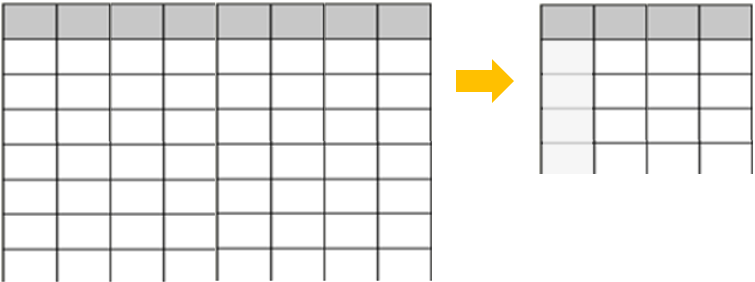
278. Your organization might decide to use aggregations in their semantic models for the following reasons:

• If you are dealing with a large amount of data (big data), aggregations will provide better query performance and help you analyze and reveal the insights of this large data. Aggregated data is cached and, therefore, uses a fraction of the resources that are required for detailed data.
• If you are experiencing a slow refresh, aggregations will help you speed up the refresh process. The smaller cache size reduces the refresh time, so data gets to users faster. Instead of refreshing what could be millions of rows, you would refresh a smaller amount of data instead.
• If you have a large semantic model, aggregations can help you reduce and maintain the size of your model.
• If you anticipate your semantic model growing in size in the future, you can use aggregations as a proactive step toward future proofing your semantic model by lessening the potential for performance and refresh issues and overall query problems.

279. During your performance review, you identified that the previous developer did not use aggregations in the semantic model, so you now want to create some aggregations for the sales data to reduce the file size and further optimize the performance.

280. Two ways to create aggregation –

• If you have access to the database, you could create a table with the aggregation and then import that table into Power BI Desktop.
• If you have access to the database, you could create a view for the aggregation and then import that view into Power BI Desktop.
• In Power BI Desktop, you can use Power Query Editor to create the aggregations step-by-step.

280. steps to follow

1. select all the columns that you need to choose by choose columns
2. under advanced option in query editor, select group by. Seelct order date.
3. provide aggregation operation for each fact columns
4. the number of rows reduced from 999 to 30.
5. Remember, you started with over 999 rows. Using aggregation has significantly reduced the number of rows in your semantic model, which means that Power BI has less data to refresh and your model should perform better.

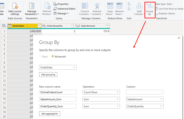
281. Manage aggregations –  In the Fields pane, right-click the table and then select Manage aggregations.

Automatic aggregations use state-of-the-art machine learning (ML) to continuously optimize DirectQuery semantic models for maximum report query performance. 

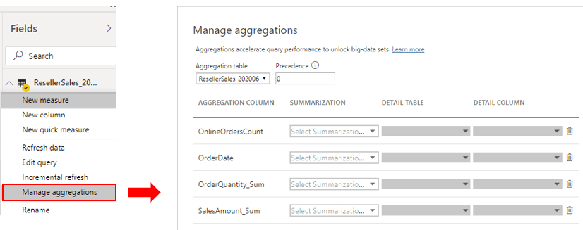
282. Advantages of automatic aggregations in Direct query – With DirectQuery, each time a model user opens a report or interacts with a report visualization, Data Analysis Expressions (DAX) queries are passed to the query engine and then to the backend data source as SQL queries. The data source must calculate and return results for each query. Compared to import mode models stored in-memory, DirectQuery data source round trips can be both time and process intensive, often causing slow query response times in report visualizations.

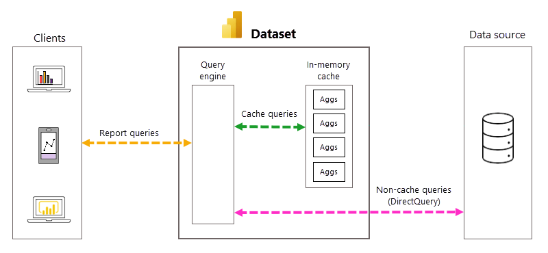
283. A working relationship can be created as long as there is at least one common column between them.

284. The benefit of analyzing the metadata is that you can clearly identify data inconsistences with your semantic model.

285. By default, a data model has no roles. A data model without roles means that users (who have permission to query the data model) have access to all model data.

286. You can create, validate, and manage roles in Power BI Desktop.

287. For Azure Analysis Services or SQL Server Analysis Services models, you can create, validate, and manage roles by using

288. RLS – Rule expressions are evaluated within row context. Row context means the expression is evaluated for each row using the column values of that row. When the expression returns TRUE, the user can “see” the row.

289. The following steps explain how Power BI enforces the rule. It:

1. Filters the Region table, resulting in one visible row (for Midwest).
2. Uses the model relationship to propagate the Region table filter to the State table, resulting in 14 visible rows (the Midwest region comprise 14 states).
3. Uses the model relationship to propagate the State table filter to the Sales table, resulting in thousands of visible rows (the sales facts for the states that belong to the Midwest region).

290. Disadvantages of Static Row level security –

Defining static rules is simple and effective.

Consider using them when you need to create only a few of them, as might be the case at Adventure Works where there are only six US regions.

However, be aware of disadvantages: setting up static rules can involve significant effort to create and set up.

It would also require you to update and republish the dataset when new regions are onboarded.

If there are many rules to set up and you anticipate adding new rules in the future, consider creating dynamic rules instead.

291. Dynamic rules use specific DAX functions that return environmental values (as opposed to constants). Environmental values are returned from three specific DAX functions:

• USERNAME or USERPRINCIPALNAME – Returns the Power BI authenticated user as a text value.
• CUSTOMDATA – Returns the CustomData property passed in the connection string. Non-Power BI reporting tools that connect to the dataset by using a connection string can set this property, like Microsoft Excel.

292. Be aware that the USERNAME function returns the user in the format of DOMAIN\username when used in Power BI Desktop.

However, when used in the Power BI service, it returns the format of the user’s User Principal Name (UPN), like username@adventureworks.com.

Alternatively, you can use the USERPRINCIPALNAME function, which always returns the user in the user principal name format.

293. Defining dynamic rules is simple and effective when a model table stores username values. They allow you to enforce a data-driven RLS design. For example, when salespeople are added to, or removed from, the AppUser table (or are assigned to different regions), this design approach just works.

294. Validate roles – When you create roles, it’s important to test them to ensure they apply the correct filters. For data models created in Power BI Desktop, there’s the View as function that allows you to see the report when different roles are enforced, and different username values are passed.

295. Role mappings must be set up in advance of users accessing Power BI content. Role mapping involves assigning Microsoft Entra security objects to roles. Security objects can be user accounts or security groups.

296. When possible, it’s a good practice to map roles to security groups. That way, there will be fewer mappings, and you can delegate the group membership management to the network administrators.

297. For Power BI Desktop developed models, role mapping is typically done in the Power BI service. For Azure Analysis Services or SQL Server Analysis Services models, role mapping is typically done in SSMS.

298. Important links on RLS

• Row-level security (RLS) with Power BI
• Row-level security (RLS) guidance in Power BI Desktop

299. Use single sign-on (SSO) for DirectQuery sources – You can create a DirectQuery model that connects to this database without roles and publish it to the Power BI service. When you set the data source credentials in the Power BI service, you enable SSO. When report consumers open Power BI reports, Power BI passes their identity to the data source. The data source then enforces RLS based on the identity of the report consumer.

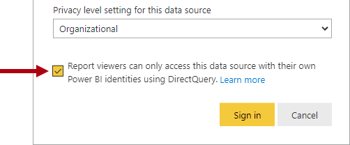
300. Calculated tables and calculated columns that reference a DirectQuery table from a data source with SSO authentication aren’t supported in the Power BI service.

301. Object-level security (OLS) can restrict access to specific tables and columns, and their metadata. Typically, you apply OLS to secure objects that store sensitive data, like employee personal data.

302. When Power BI enforces OLS, not only does it restrict access to tables and columns, but it can also secure metadata. When you secure metadata, it’s not possible to retrieve information about secured tables and columns by using Dynamic Management Views (DMVs).

303. Tabular models can hide tables and columns (and other objects) by using a perspective.

304. A perspective defines viewable subsets of model objects to help provide a specific focus for report authors. Perspectives are intended to reduce the complexity of a model, helping report authors find resources of interest.

305. However, perspectives aren’t a security feature because they don’t secure objects. A user can still query a table or column even when it’s not visible to them.

306. The table includes columns that store employee name, phone, email address, and salary. While general report consumers can see employee name and contact details, they must not be able to see salary values. Only senior Human Resources staff are permitted to see salary values. So, the data modeler used OLS to grant access to the salary column only to specific Human Resources staff.

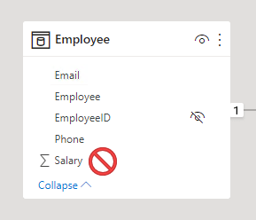
307. OLS is a feature inherited from Azure Analysis Services (AAS) and SQL Server Analysis Services (SSAS). The feature is available in Power BI Premium to provide backward compatibility for models migrated to Power BI. For this reason, it’s not possible to completely set up OLS in Power BI Desktop.

308. To set up OLS, you start by creating roles. You can create roles in Power BI Desktop in the same way you do when setting up RLS. Next, you need to add OLS rules to the roles. This capability isn’t supported by Power BI Desktop, so you’ll need to take a different approach.

309. Power BI Pro is required to use RLS features

310. You add OLS rules to a Power BI Desktop model by using an XML for Analysis (XMLA) endpoint. XMLA endpoints are available with Power BI Premium, and they provide access to the Analysis Services engine in the Power BI service.

311. You can use XMLA endpoint-enabled APIs for scripting, such as Tabular Model Scripting Language (TMSL) or the PowerShell SqlServer module. Or you can use a client tool, like SSMS. There are third-party tool options too, like Tabular Editor, which is an open-source tool for creating, maintaining, and managing models.

312.

By default, all model tables and columns aren’t restricted. You can set them to None or Read. When set to None, users associated with the role can’t access the object. When set to Read, users associated with the role can access the object. When you’re restricting specific columns, ensure the table isn’t set to None.

Once you’ve added the OLS rules, you can publish the model to the Power BI service. Use the same process for RLS to map accounts and security groups to the roles.

313. In a Power BI report, when a user doesn’t have permission to access a table or column, they’ll receive an error message. The message will inform them that the object doesn’t exist.

314. Consider carefully whether OLS is the right solution for your project. When a user opens a Power BI report that queries a restricted object (for them), the error message could be confusing and will result in a negative experience. To them, it looks like the report is broken. A better approach might be to create a separate set of models or reports for the different report consumer requirements.

315. Message when RLS is restricted for specific role.

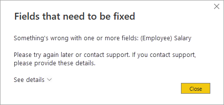
316. There are restrictions to be aware of when implementing OLS.

You can’t mix RLS and OLS in the same role. If you need to apply RLS and OLS in the same model, create separate roles dedicated to each type. Also, you can’t set table-level security if it breaks a relationship chain.

For example, if there are relationships between tables A and B, and B and C, you can’t secure table B. If table B is secured, a query on table A can’t transit the relationships between table A and B, and B and C. In this case, you could set up a separate relationship between tables A and C.

317. Apply good modeling practices –

• Strive to define fewer datasets (data models) with well-designed roles.
• Strive to create fewer roles by using dynamic rules. A data-driven solution is easier to maintain because you don’t need to add new roles.
• When possible, create rules that filter dimension tables instead of fact tables. It will help to deliver faster query performance.
• Validate that the model design, including its relationships and relationship properties, are correctly set up.
• Use the USERPRINCIPALNAME function instead of USERNAME function. It provides consistency when validating the roles in Power BI Desktop and the Power BI service.
• Rigorously validate RLS and OLS by testing all roles.
• Ensure that the Power BI Desktop data source connection uses the same credentials that will be applied when set up in the Power BI service.

318. An RLS role with a static rule can’t filter model data based on the employee table in the database.

319. It’s efficient to apply rules to dimension tables. Power BI filters the dimension tables (that usually have a small number of rows) and uses model relationships to propagate those filters to fact tables (that contain millions of rows).