How to Create a Task Tracker in Excel in Less Than One Minute

In this post, you will learn how to quickly build a task tracker in Excel using checkboxes, formulas, and progress bars, all in under one minute!

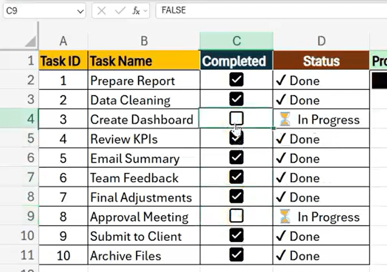
Task Data – Your Excel sheet has the following columns:
👉 Task ID
👉 Task Name
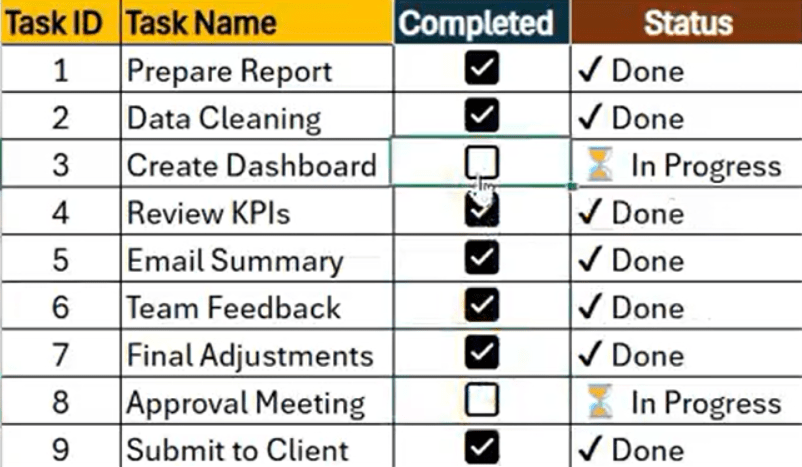
👉 Completed (with checkboxes)
👉 Progress Bar
👉 Percentage Completed
👉 Conditional Formatting

Step 1: Add Checkboxes
👉 Go to Insert tab click Check Box (Under Controls).
🖱️ Drag to draw checkboxes inside cells C2 to C11.



Step 2: Show Task Status Using a Formula
Type the following formula in cell D2 and drag it down to D11:
=IF(C2=TRUE, “✔ Done”, “⏳ In Progress”)
This will show either a checkmark for completed tasks or an hourglass for pending ones.


Step 3: Create a Visual Progress Bar
To show how much is completed, use this formula in cell E2:
=REPT(“█”, COUNTIF(C$2:C$11, TRUE)) & REPT(“░”, COUNTA(C$2:C$11)-COUNTIF(C$2:C$11, TRUE))
This bar will grow as you check more boxes, giving a visual feel of your progress!

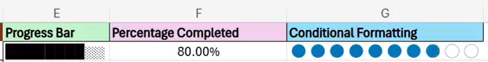
Step 4: Show Percentage Completed
In cell F2, use this formula:
=COUNTIF(C2:C11, TRUE)/COUNTA(C2:C11)
Format this cell as Percentage to show something like 40% completed.


Step 5: Make It Look Better with Conditional Formatting
Go to the column with your REPT formula (like G2).
Apply Conditional Formatting to change colors based on completion.
You can also swap the REPT symbols with emojis for more style:
=REPT(“🔵”, COUNTIF(C$2:C$11, TRUE)) & REPT(“⚪”, COUNTA(C$2:C$11)-COUNTIF(C$2:C$11, TRUE))
This shows a blue and white bubble bar to track your progress.