Filter , Sort & Sequence Excel Functions

It’s a tremendous compounding effect when you learn excel formulas everyday. Here’s drafting the explanation about the three major excel functions with examples. You can download the excel from here for reference.

1. Filter Function:

Filter function is very handy when you want to filter the specific part of the table data. Lets see both single and multiple conditions using Filter function.

Category	Couches	Recliners	Coffee Tables	End Tables	Total
Retail	4,310	4,960	3,420	4,510	17,200
Wholesale	2,340	2,750	2,980	3,550	11,620
Internet	3,420	4,030	3,840	4,380	15,670

Basic FILTER formula – Single condition

=FILTER(Sales1,Sales1[Recliners]>=3000)

Category	Couches	Recliners	Coffee Tables	End Tables	Total
Retail	4310	4960	3420	4510	17200
Internet	3420	4030	3840	4380	15670

Basic FILTER formula – Multiple condition

If you want to extract data based on both the two conditions, then use * . If based one either of the one condition, then use ” + ” .

=FILTER(Sales1,Sales1[Recliners]>=3000 * Sales1[Coffee Tables]>=2000)

=FILTER(Sales1,Sales1[Recliners]>=3000 + Sales1[Coffee Tables]>=2000)

Category	Couches	Recliners	Coffee Tables	End Tables	Total
Retail	4310	4960	3420	4510	17200
Wholesale	2340	2750	2980	3550	11620
Internet	3420	4030	3840	4380	15670

Filter duplicates:

If you want to extract the duplicate rows, then use countifs function. The below table is filtering all the duplicates on the field Category and Profit.

Category	Couches	Recliners	Coffee Tables	End Tables	Total	Profit
Retail	4,310	4,960	3,420	4,510	17,200	Yes
Wholesale	2,340	2,750	2,980	3,550	11,620	Yes
Internet	3,420	4,030	3,840	4,380	15,670	No
Internet	3,420	4,030	3,840	4,380	15,670	No
Wholesale	1,240	1,650	1,880	2,450	10,520	Yes
Wholesale	2,340	2,750	2,980	3,550	11,620	Yes
Wholesale	2,340	2,750	2,980	3,550	11,620	Yes

=FILTER(Sales2,COUNTIFS(Sales2[Category],Sales2[Category],Sales2[Profit],Sales2[Profit])>1)

Wholesale	2340	2750	2980	3550	11620	Yes
Internet	3420	4030	3840	4380	15670	No
Internet	3420	4030	3840	4380	15670	No
Wholesale	1240	1650	1880	2450	10520	Yes
Wholesale	2340	2750	2980	3550	11620	Yes
Wholesale	2340	2750	2980	3550	11620	Yes

2. Filter & Sort Function:

You can extract the data using filter function and sort the data as well. To do so, lets take a table as below.

Item	Qty.
Apples	38
Cherries	29
Grapes	31
Lemons	34
Melon	26
Oranges	36
Peaches	25
Pears	40

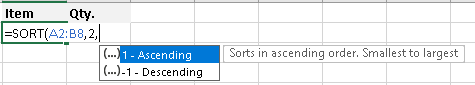
SORT(FILTER(array, criteria_range=criteria), [sort_index], [sort_order], [by_col])

The important thing to notice in this formula is that you do not need to press Ctrl + Shift + Enter to convert it as an Array. Just type a formula in the upper most cell and hit the Enter key.

Sort Index -Depicts the column number which you want to sort.

Sort Order – You can sort the data either ascending or descending order. By default it will be sorted by ascending order.

=SORT(FILTER(A2:B9, B2:B9>=30), 2)

Item	Qty.
Grapes	31
Lemons	34
Oranges	36
Apples	38
Pears	40

3. Index, Sort & Sequence Function:

When analyzing huge amount of information, you need to extract a certain number of top values. With dynamic array functions, you can easily sort and also display Top N or Bottom N values.

INDEX(SORT(…), SEQUENCE(n), {column1_to_return, column2_to_return, …})

Region	Item	Qty.
East	Lemons	36
East	Grapes	31
North	Cherries	29
North	Grapes	27
North	Peaches	25
South	Pears	40
South	Apples	38
South	Oranges	36
South	Cherries	28
West	Lemons	34
West	Apples	30
West	Oranges	29

=INDEX(SORT(A2:C13,3,-1),SEQUENCE(3),{2,3})

In the above formula,

• A2:C13 – denotes the data set
• 3 – denotes the column Qty
• -1 – denotes the descending order
• Sequence function (3) – displays the top 3 values
• {2,3} – returns the column Items and Qty.

Item	Qty.
Pears	40
Apples	38
Lemons	36

Hope you find it useful. Catch you in the next post.