A-Z of Power Query

Create Low Code Automated Dashboard

Are you finding difficult to learn VBA – Macros like me?

Are you taking more time to clean & transform your data like me?

Are you looking for “Low code options to perform ETL process like me?

Bored of doing repetitive tasks in Excel?

Power Query & Power Pivot is the MUST-KNOW feature

It gives more POWER within excel from data transformation to data analysis to data visualization, as it is proven that 70% of the time is spent in collecting, cleaning, transforming the data. ETL process is a very common steps involved while reporting which stands for Extract, Transform & Load the data.

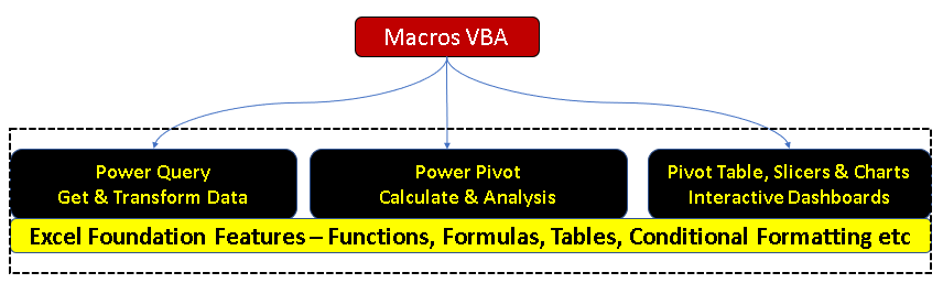
Combination of Power Query & Power Pivot = POWER BI

Listing the key features of Power Query one must know. Most of the features are done by just Click of a Button. We don’t need to repeat these every month. Power Query will automatically update the calculations once the datasets are refreshed. This post is a good bookmark for myself 🙂 Stay tuned for post about Power Pivot!

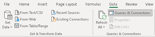
There is no Addin to be installed for Power Query. This is a free add-in as part of Excel 2010 onwards. You can find all the Power Query options under the Data menu.

Know your sources of data -Live update:

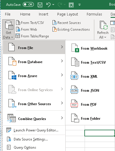
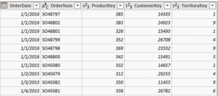
You should know that within excel from where you can import the data from any source. Also, You can create your own query or table. Be it a simple range of cells, SQL, Azure, SharePoint, any website link, XML, CSV, Text, or even from PDF, you can import the data from anywhere.

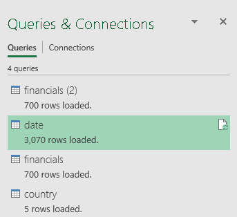
Importing the worksheets or workbooks to get the combined data can be done in no time now. You can place your dump files in a folder and import the folder. Every month, just replacing the files and refreshing will automatically refresh your datasets.

Load to Data model :

Excel cannot exceed the limit of 1,048,576 rows and 16,384 columns. So ensure you query your data i.e. load to the data model and not to the worksheet in order to avoid the truncation of the cells in case of a huge amount of data. Else you can import the combined data into the worksheet.

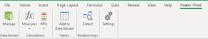
Install the Power Pivot Addin:

Like Power Query, Power Pivot helps to perform the calculations, analyze the data and produce data for effective decision making. You can create calculated fields, create relationships, find KPI’s and even DAX functions can be applied.

Merge Columns / Tables:

You can merge the columns or two tables in the power query. When we say merge, it is not just copied and paste. The Merge button is an equivalent of JOIN in SQL. It’s also similar to the LOOKUP/Index/Match function in Excel.

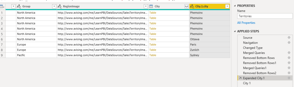
Below we have merged two simple columns, the Month and Year, and created a new column. Similarly, When two datasets are merged or joined, additional columns are added. But it is important to be cautious when you have duplicates as behavior is different when multiple matches are found.

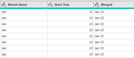
After merging, don’t forget to click expand to add the columns in the existing table.

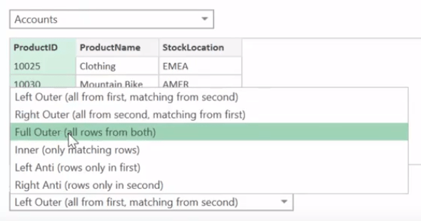
There are 6 types of Joins. Depending on the data, you can select the option appropriately.

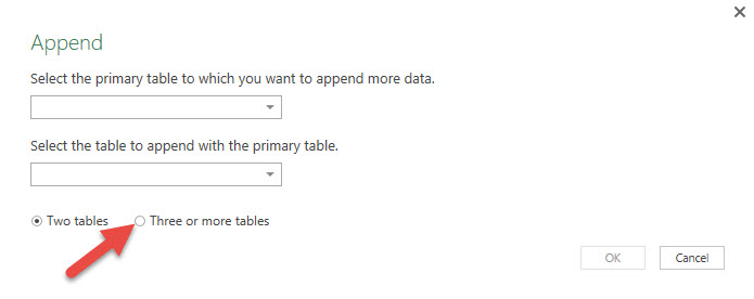
Append Queries:

When you have additional rows of data that you’d like to add to an existing table, you append the query. When you have two sets of tables with the same fields depicting the sales figures for two different years, you can append them into a single table with just one click.

Consolidate Multiple Excel sheets:

If you have multiple worksheets that are in the same format and their differences are their values and dates (e.g. January List, February List, March List, etc.), then we can easily consolidate all the worksheets into one.

Create a Custom Calendar in Power Query

Most of the time, we deal with time-related metrics, and creating a calendar query will help you to analyze your data on a daily, weekly, monthly, quarterly, or yearly basis.

Insert a blank query and Type in the code      =List.Dates

An easy method to create a custom calendar is to copy-paste the following code in a blank query. (Source)

let
Source = List.Dates,
#"Invoked FunctionSource" = Source(#date(2015, 1, 1), Duration.Days(DateTime.Date(DateTime.FixedLocalNow()) - #date(2015,1,1)), #duration(1, 0, 0, 0)),
#"Table from List" = Table.FromList(#"Invoked FunctionSource", Splitter.SplitByNothing(), null, null, ExtraValues.Error),
#"Added Index" = Table.AddIndexColumn(#"Table from List", "Index", 1, 1),
#"Renamed Columns" = Table.RenameColumns(#"Added Index",{{"Column1", "Date"}}),
#"Added Custom" = Table.AddColumn(#"Renamed Columns", "Year", each Date.Year([Date])),
#"Added Custom1" = Table.AddColumn(#"Added Custom", "Month Number", each Date.Month([Date])),
#"Added Custom2" = Table.AddColumn(#"Added Custom1", "Day", each Date.Day([Date])),
#"Added Custom3" = Table.AddColumn(#"Added Custom2", "Day Name", each Date.ToText([Date],"ddd")),
#"Added Custom4" = Table.AddColumn(#"Added Custom3", "Month Name", each Date.ToText([Date],"MMM")),
#"Reordered Columns" = Table.ReorderColumns(#"Added Custom4",{"Date", "Index", "Year", "Month Number", "Month Name", "Day", "Day Name"}),
#"Added Custom5" = Table.AddColumn(#"Reordered Columns", "Quarter Number", each Date.QuarterOfYear([Date])),
#"Duplicated Column" = Table.DuplicateColumn(#"Added Custom5", "Year", "Copy of Year"),
#"Renamed Columns1" = Table.RenameColumns(#"Duplicated Column",{{"Copy of Year", "Short Year"}}),
#"Changed Type" = Table.TransformColumnTypes(#"Renamed Columns1",{{"Short Year", type text}}),
#"Split Column by Position" = Table.SplitColumn(#"Changed Type","Short Year",Splitter.SplitTextByRepeatedLengths(2),{"Short Year.1", "Short Year.2"}),
#"Changed Type1" = Table.TransformColumnTypes(#"Split Column by Position",{{"Short Year.1", Int64.Type}, {"Short Year.2", Int64.Type}}),
#"Removed Columns" = Table.RemoveColumns(#"Changed Type1",{"Short Year.1"}),
#"Renamed Columns2" = Table.RenameColumns(#"Removed Columns",{{"Short Year.2", "Short Year"}}),
#"Added Custom6" = Table.AddColumn(#"Renamed Columns2", "Quarter Year", each Number.ToText([Short Year]) & "Q" & Number.ToText([Quarter Number],"00")),
#"Reordered Columns1" = Table.ReorderColumns(#"Added Custom6",{"Index", "Date", "Day", "Day Name", "Month Number", "Month Name", "Quarter Number", "Quarter Year", "Short Year", "Year"}),
#"Changed Type2" = Table.TransformColumnTypes(#"Reordered Columns1",{{"Date", type date}, {"Day", Int64.Type}, {"Index", Int64.Type}, {"Month Number", Int64.Type}, {"Quarter Number", Int64.Type}, {"Month Name", type text}, {"Quarter Year", type text}, {"Year", Int64.Type}})
in
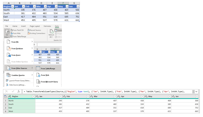
#"Changed Type2"

Create Pivot Columns:

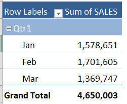
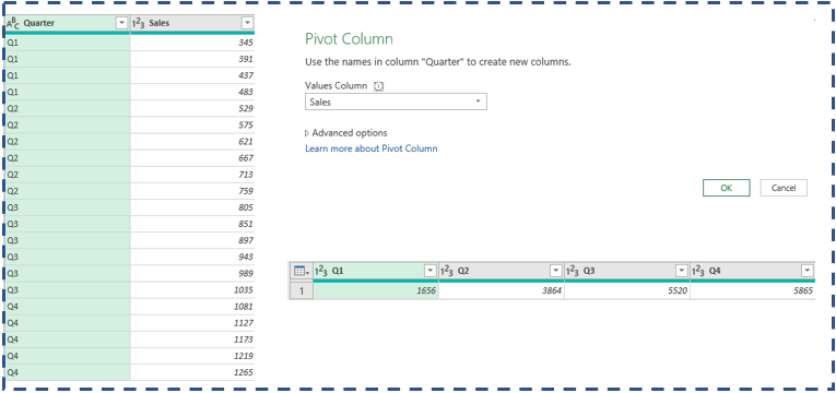
This amazing feature of Power Query has hundreds of benefits. We can use it for a data source that has too many numbers of columns and rows. To simplify your data and aggregate them together we can Pivot the huge data table using Power Query Editor in excel. Below shows the sample data which can be aggregated using Pivot column.

Pivoting is just a process of turning distinct row values into their own columns and, whereas Unpivoting is turning columns into rows.

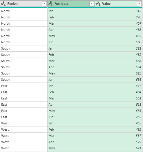
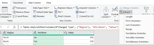
Unpivot the Data:

Pivot Tables are great when you want to analyze a huge amount of data in seconds. It also allows you to quickly create different views of data by simply dragging and dropping. Most of the time, the source data is not pivot friendly. But using unpivot columns feature in Power query, see below how the pivot-friendly table can be created. There are three different features an each give result based on the required output.

• Unpivot columns
• Unpivot other columns
• Unpivot only selected columns

First, Add the data to data model.

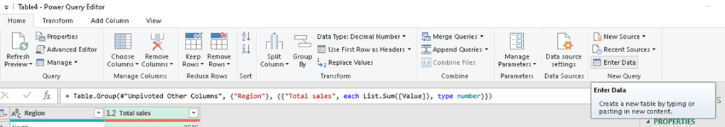
Right click on column Region, select “unpivot other columns”, will create a table as below:

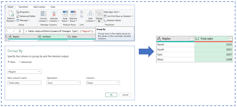
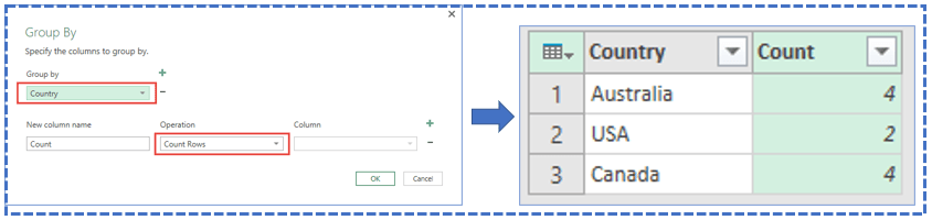
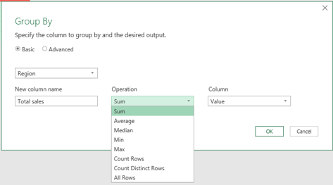
Group By / Group rows and get counts

Now that we have unpivot the data, now we would like to further group the data as below.

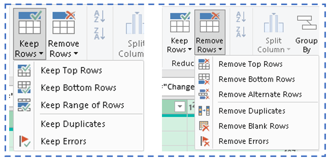
Keep Rows / Remove Rows Feature:

There are multiple times, when you want to delete certain rows from your data. Power Query has the below options, which you can perform at just click of a button.

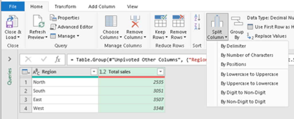
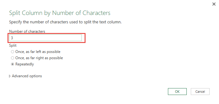
Split column by No of characters:

There are various options to play around the text columns. “Split column” feature in Power query has lot to do.

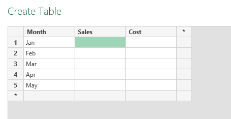
Create Data Table directly in Power Query:

Enter Data option in Power query lets you create a table of data in minutes. You don’t need to import from anywhere.

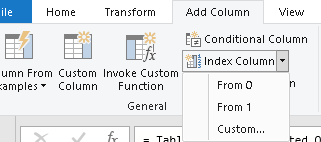
Add index columns in Just one Click:

When you have loads of rows in your data, at times, you wanted to have an index which will help in many calculations. You can use INDEX to retrieve individual values or entire rows and columns. INDEX is often used with the MATCH function, where MATCH locates the position and feeds a position to INDEX.

Transform Data with various features:

The options available in Transform Menu are

1. Group data by
2. Use first row as Headers
3. Transpose
4. Reverse Rows
5. Count Rows
6. Change the Data type
7. Replace value in data sets
8. Split column
9. Merge column
10. Pivot & Unpivot columns
11. Date & Time related functions
12. Format the data

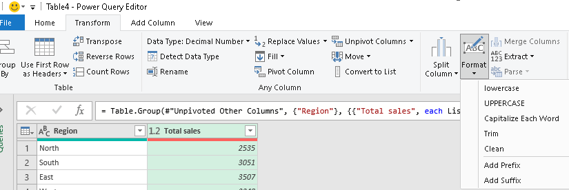
Format the Text Data:

Tired of writing formulas for converting your text. See the below options that you got in Power Query, in just click of a button.

Simple Extract Functions:

Just extract the data however you want in just clicks.

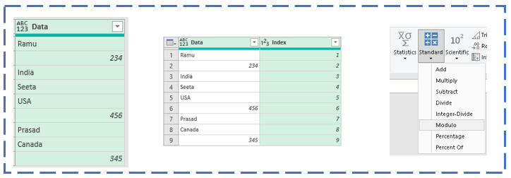
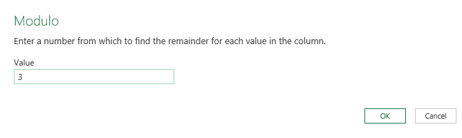
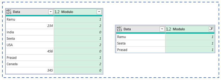
Modulo calculation in Power Query:

Say you have a column with mixed set of data and you want to filter only Names. First add index column, then click Modulo from Standard drop-down menu. Select the number of rows you want to repeat.

Happy Querying 🙂