Excel Magic Function XLOOKUP() with 10 Examples

Long awaited Xlookup finally arrived.

If you have been using VLOOKUP or INDEX/MATCH, I am sure you’ll love the flexibility that the XLOOKUP function provides.

XLOOKUP is a function that allows you to quickly look for a value in a dataset (vertical or horizontal) and return the corresponding value in some other row/column.

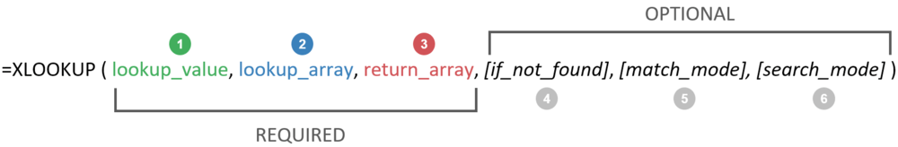
=XLOOKUP(lookup_value, lookup_array, return_array, [if_not_found], [match_mode], [search_mode]) 

XLOOKUP function has 6 arguments (3 mandatory and 3 optional)

lookup_value – the value that you’re looking for

lookup_array – the array in which you’re looking for the lookup value

return_array – the array from which you want to fetch and return the value (corresponding to the position where the lookup value is found)

[if_not_found] – the value to return in case the lookup value is not found. In case you don’t specify this argument, a #N/A error would be returned

[match_mode] – Here you can specify the type of match you want:

• 0 – Exact match, where the lookup_value should exactly match the value in the lookup_array. This is the default option.
• -1 – Looks for the exact match, but if it’s found, returns the next smaller item/value
• 1 – Looks for the exact match, but if it’s found, returns the next larger item/value
• 2 – To do partial matching using wildcards (* or ~)

[search_mode] – Here you specify how the XLOOKUP function should search the lookup_array

Another notable improvement with XLOOKUP is that now there are four match modes (VLOOKUP has 2 and MATCH has 3).

• 1 – This is the default option where the function starts looking for the lookup_value from the top (first item) to the bottom (last item) in the lookup_array
• -1 – Does the search from bottom to top. Useful when you want to find the last matching value in the lookup_array
• 2 – Performs a binary search where the data needs to be sorted in ascending order. If not sorted, this can give errors or wrong results
• -2 – Performs a binary search where the data needs to be sorted in descending order. If not sorted, this can give errors or wrong results

Example 1: Simple Xlookup – Vertical Lookup

Simple example only with mandatory values.

=XLOOKUP(F2,A2:A15,B2:B15)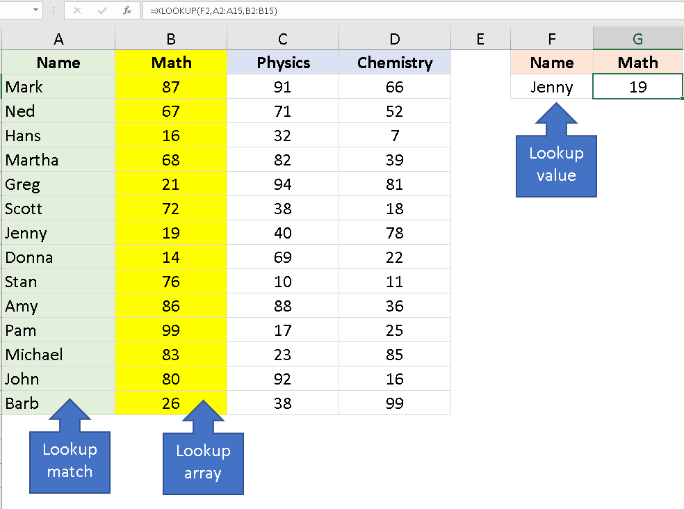

Example 2: Array Range – Fetch the entire record

In this case, I don’t want to just fetch Greg’s score in Math. I want to get the scores in all the subjects in the same order. Then use ARRAY RANGE.

The formula returns the entire row from the return_array.

You need to enter the formula only in the G column. The values in H & I, will be populated automatically.

The only thing to note is that you can edit the formula. It would be greyed out.

This is useful feature, so that you dont want to change column number just like in VLOOKUP().

=XLOOKUP(F2,A2:A15,B2:D15)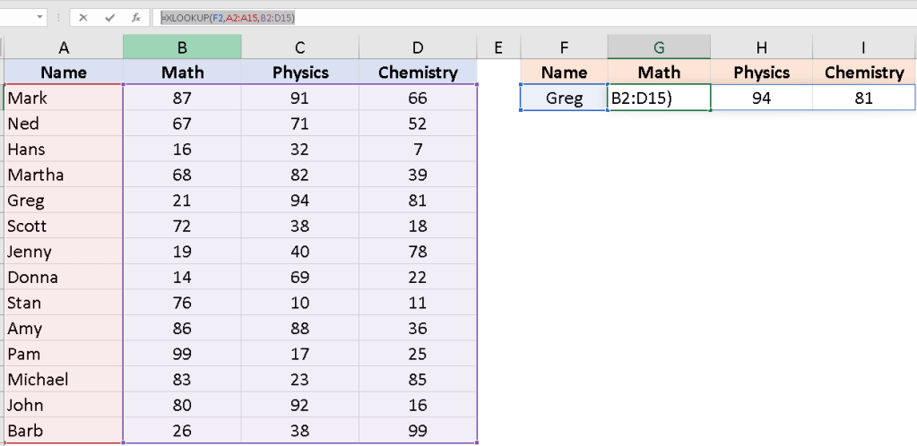

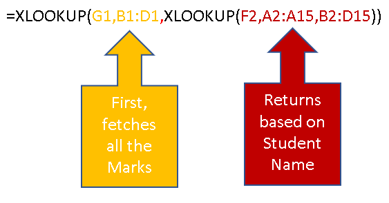
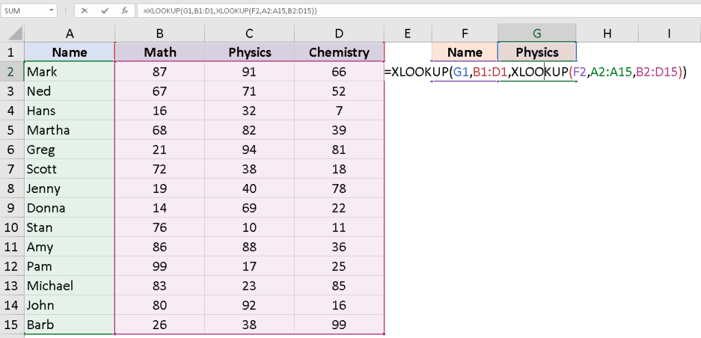
Example 3: Two way lookup

If you have a lookup values both in the horizontal and vertical directions, then use like below format.

This does the same that was, until now, achieved using the INDEX and MATCH combo.

=XLOOKUP(G1,B1:D1,XLOOKUP(F2,A2:A15,B2:D15))

The benefit of this two-way lookup is that the result is independent of the student name of the subject name. 

Example 4: Lookup Value is Not Found

If the lookup value s not found, then you use the optional parameter. Either you can input the text or give cell reference.

=XLOOKUP(F2,A2:A15,B2:B15,"Did Not Appear")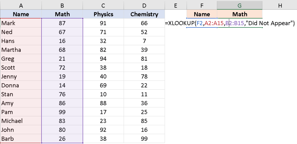

Example 5: Nested Xlookup

You can use it for about 10 Nested Xlookup functions. The below examples show two tables.

=XLOOKUP(A12,A2:A8,B2:B8,XLOOKUP(A12,F2:F8,G2:G8))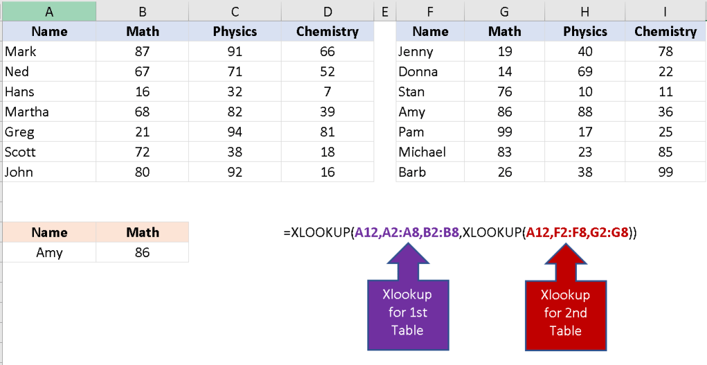

Example 6: Last Matching Value

Search mode is used if you want to fetch the last found value.

Suppose you have the dataset as shown below and you want to check when was the last person hired in each department and what was the hire date.

=XLOOKUP(F1,$B$2:$B$15,$C$2:$C$15,,,-1)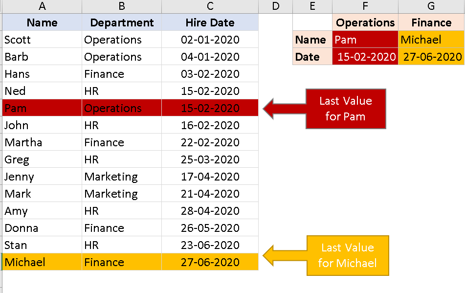

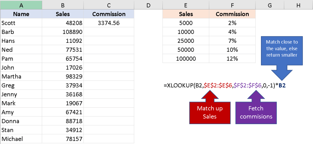
Example 7: Approximate Match

• 0 – Exact match, where the lookup_value should exactly match the value in the lookup_array. This is the default option.
• -1 – Looks for the exact match, but if it’s found, returns the next smaller item/value
• 1 – Looks for the exact match, but if it’s found, returns the next larger item/value
• 2 – To do partial matching using wildcards (* or ~)

Lets recall the formula once.

=XLOOKUP(lookup_value, lookup_array, return_array, [if_not_found], [match_mode], [search_mode]) 

If I need to find the commission based on sales value, then

'=XLOOKUP(B2,$E$2:$E$6,$F$2:$F$6,0,-1)*B2

” – 1 ” is used to match close to the value, if not returns the smallest number.

Example 8: Horizontal Lookup

Say, I want to fetch the value in the horizontal dataset.

If i want to fetch the marks based on the name and subject in the horizontal direction, then use the formula below.

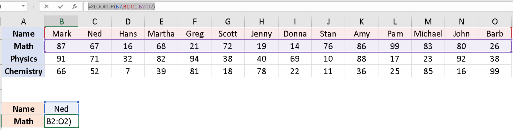
=XLOOKUP(B7,B1:O1,B2:O2)

First, lookup for the name B1:O1

then Subject row, B2:O2

The value will be fetched based on the name.

Example 9: Conditional Lookup

Suppose , you want to find the no of students who scored more than 80. Then, use the below formula.

=COUNTIF(XLOOKUP(G1,$B$1:$D$1,$B$2:$D$15),">80")

Step 1 – First find the max score using the xlookup.

MAX(XLOOKUP(G1,$B$1:$D$1,$B$2:$D$15)

Then use that within another xlookup to fetch the name of the student based on the maximum score.

'=XLOOKUP(MAX(XLOOKUP(G1,$B$1:$D$1,$B$2:$D$15)),XLOOKUP(G1,$B$1:$D$1,$B$2:$D$15),$A$2:$A$15)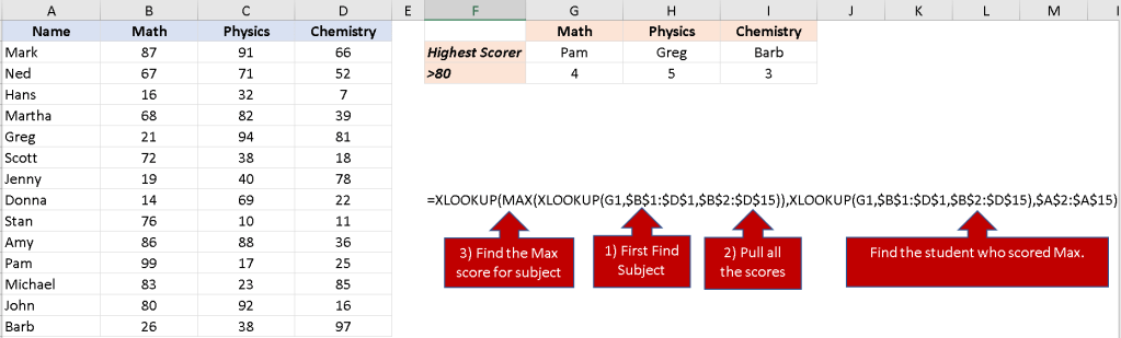

Example 10: Xlookup with Wild Card

When the lookup value is not same, then you can use wildcard char.

Say, I want to fetch the M.Cap value based on company name which is not same in the data table.

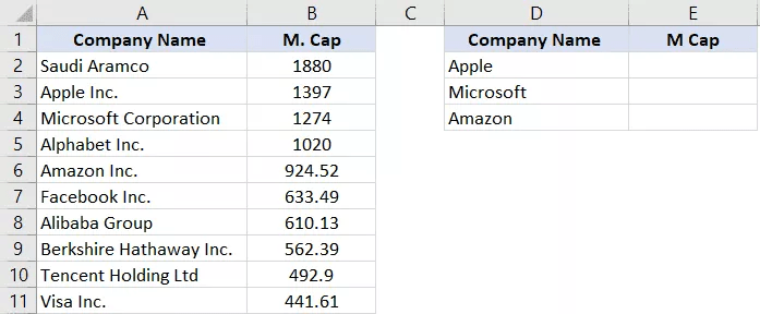
=XLOOKUP("*"&D2&"*",$A$2:$A$11,$B$2:$B$11,,2)

The formula “*”&D2&”*” tells that lookup for the company name that contains the exact match of the lookup value ie Apple here.

The number “2”, tells To do partial matching using wildcards (* or ~)

Similarly, if I want to calculate the last company name and its M.cap value, then use

=XLOOKUP("*",A2:A11,A2:A11,,2,-1)

2 – To do partial matching using wildcards (* or ~) & -1 t do bottom to top direction.

Conclusion

Below is the alternative for Xlookup if you get struck in the formula.

Use CASE	XLOOKUP Alternative
Regular lookups	Use VLOOKUP or INDEX+MATCH
Lookup in the middle, get value from elsewhere	Use INDEX+MATCH
Get the last item (lookup from last)	Lookup last value trick
2-way lookups (lookup row & column intersection)	Use INDEX MATCH MATCH
IF not found option	Use IFERROR

Hope you found this tutorial useful!