Excel Advanced Formulas

Excel formulas are like bread and butter for anyone being in PMO. Summarising the important formulas one should be aware of, along with examples. It was a good recap for me.

The below is the list of functions we are going learn together.

1. AND(), OR(), NOT()
2. IF() and IFS()
3. SWITCH()
4. SUMIF() SUMIFS(),
5. AVERAGEIF() / AVERAGEIFS()
6. COUNT() and COUNTIF()
7. MAXIFS() and MINIFS()
8. VLOOKUP() and HLOOKUP()
9. MATCH() and INDEX()
10. DATE()
    • NOW()
    • TODAY()
    • WEEKDAY()
    • WORKDAY()
    • Networkdays()
11. CONSOLIDATE()

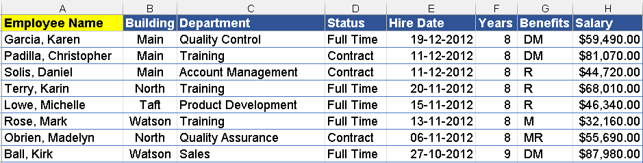
Excel Function 1 – AND(), OR(), NOT() as Nested Function

The main difference between these is the result returns based on the condition.

AND() — returns TRUE both sets of criteria

OR() — returns TRUE if one or both sets of criteria

NOTO — returns TRUE if is not equal to the condition

EXAMPLE:

=IF(AND(C4="Full Time"),"Yes", "No")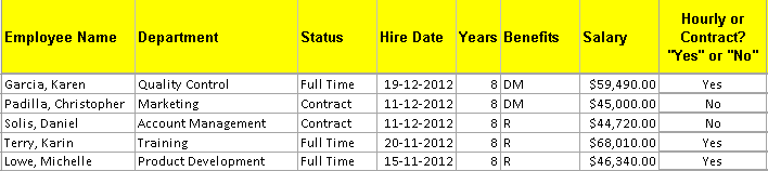

=IF(AND(B2="Marketing",G2<50000),"Increase")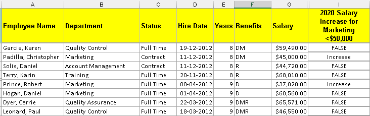

=NOT(OR(B2="Product Development",B2="Manufacturing"))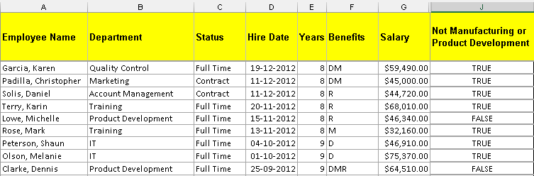

Excel Function 2- IF() and IFS() in nested functions

Nested IF in Excel is commonly used when you want to evaluate situations that have more than two possible outcomes. Nested IF function would resemble “IF(IF(IF()))”. However, this old method can be challenging and time-consuming at times.

The IFS function in Excel shows whether one or more conditions are observed and returns a value that meets the first TRUE condition. IFS is an alternative to Excel multiple IF statements and it is much easier to read in case of several conditions. Excel IFS lets you evaluate up to 127 different conditions.

EXAMPLE:

In the below example, beginning in D6, for each employee, enter “Yes” if the goal was met and “No” if it was not met.

=IF(C3>500000, "Yes", "No")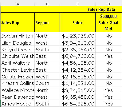

In the below example, beginning in F6, if the employee met the goal, “Good”; if the employee exceeded the goal, “Great”; if the employee did not meet the goal, “Poor”.

=IFS(C3<500000,"Poor",C3=500000,"Good",C3>500000,"Great")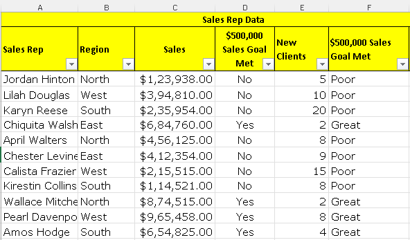

Beginning in G6, if the new client goal was met, enter “Met”; if the new client goal was exceeded, enter “Exceeded”; if the goal wasn’t met, enter “Not Met”.

=IFS(E6=5,"Met",E6>5,"Exceeded",E6<5,"Not Met")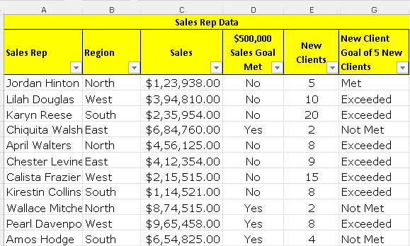

Excel Function 3 – SWITCH() in nested functions

One of the new functions available to us in Office 2019 and in Office 365 is the SWITCH function. Now, this function will compare a value against a list, and it will return the first match that it finds in that list. If no match is found, we have an optional default value that we can put in. The SWITCH function was first introduced in Excel 2016 not to replace the IF function, but instead as an alternative to nested IF formulas.

Assign a Level to each Sales Rep based on their Ranking in the Sales Department:

• <$400,000 = Rank 1:  Bronze
• <$700,000 = Rank 2:  Silver
• >$700,000 = Rank 3:  Gold

=IF(E10=1,"Bronze",IF(E10=2,"Silver","Gold"))

=SWITCH(E4,1,"Bronze",2,"Silver",3,"Gold")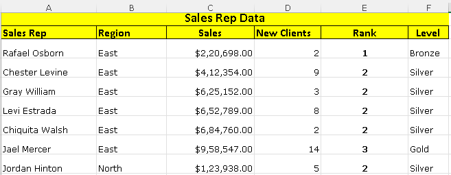

Excel Function 4 – SUMIF() SUMIFS(), AVERAGEIF() / AVERAGEIFS() functions

SUMIF() requires just one set of criteria and if that criteria is met it will fall within the range that we’ve asked Excel to sum. SUMIFS() requires two or more sets of criteria and if both of those are met it will then sum the data in the range that we’ve selected.

AVERAGEIF() and AVERAGEIFS() work exactly the same way except of course that it averages the information instead of summing.

• SUMIF() — one set of criteria
• SUMIFS() — two or more sets of criteria
• AVERAGEIF() — one set of criteria
• AVERAGEIFS() — two or more sets of criteria

=SUMIF(range, criteria, [sum_range])

=SUMIFS (sum_range, range1, criteria1, [range2], [criteria2], ...)

=SUMIF(B2:B736,"Training",G2:G736) - Total Salary for Training Employees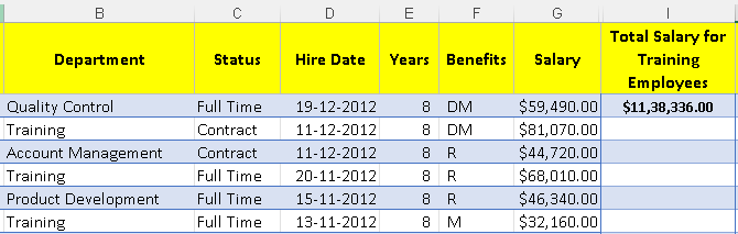

=SUMIFS(G2:G736,B2:B736,"Training",C2:C736,"Full Time") - Total Salary for Full Time Training Employees ( Two conditions)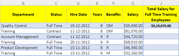 

AVERAGEIF(range, criteria, [average_range])

=AVERAGEIFS(average_range, criteria_range1, criteria1, ...)

=AVERAGEIF(B2:B736,"Training",G2:G736) - Average Years for Marketing Employees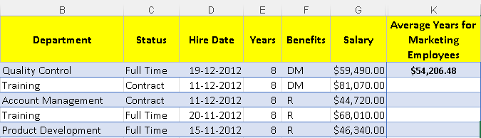

=AVERAGEIFS(G2:G736,B2:B736,"Quality Assurance",C2:C736,"Contract")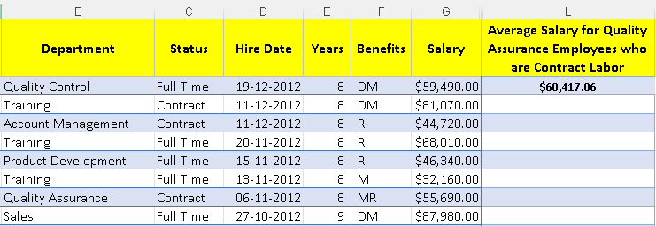

Excel Function 5 – COUNT() and COUNTIF()

The COUNTIF function is used if you just have one set of criteria, and if that criterion is met, Excel will count those records in your range. And of course, if we have more than one set of criteria, we can use COUNTIFS.

=COUNT(G4:G738) 

*Just the count of employees

=COUNTIF(B4:B738,"Training")

*How Many Training Employees?*

=COUNTIFS(B4:B738,"Training",E4:E738,">10")

*Training Employees Employed More than 10 Years*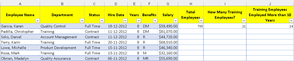

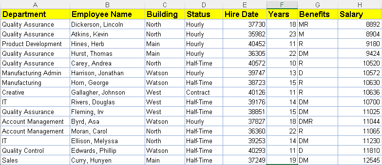
Excel Function 6 – MAXIFS() and MINIFS() in nested functions

MAXIFS() and MINIFS() are similar to MAX and MIN, but we can use them for multiple conditions.

Let’s check the syntax of the functions.

MAXIFS(max_range, criteria_range1, criteria1, [criteria_range2, criteria2], …)

MINIFS(min_range, criteria_range1, criteria1, [criteria_range2, criteria2], …)

Example:

Lets find the Largest Salary based on the condition of Account Management, Dallas Location, Full Time Status.

=MAXIFS(H2:H736,C2:C736,C728,B2:B736,"Dallas",D2:D736,"Full Time")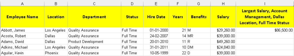

Lets find the Earliest Date of Hire based on Los Angeles Location, Full Time Status. For this, we will be using to use MINIFS.

=MINIFS(E2:E736,B2:B736,B722,D2:D736,"Full Time")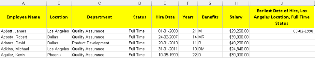

Excel Function 7 – Look up data using VLOOKUP() and HLOOKUP()

Let’s talk about two basic functions in Excel where you can look up data either vertically or horizontally.

HLOOKUP():

HLOOKUP(lookup_value, table_array, row_index_num, [range_lookup])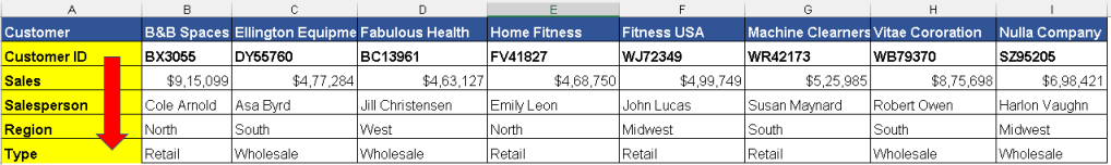

Say, I need to find the Sales and Saleperson details for each customer. As I’m drilling top to bottom, we will be using Hlookup formula here.

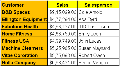
=HLOOKUP($A11,$A$1:$I$6,3,0)
where A11 is the Customer name ; 
$A$1:$I$6 is the entire data set
3 is the no of rows that need to go down, as I need sales data which is 3 row from top. 
0- Exact match

=HLOOKUP($A11,$A$1:$I$6,4,0)
where A11 is the Customer name ; 
$A$1:$I$6 is the entire data set
4 is the no of rows that need to go down, as I need salesperson data which is 4 row from top. 
0- Exact match

VLOOKUP():

Below is the sample data set.

Lets find the Department and Years with company.

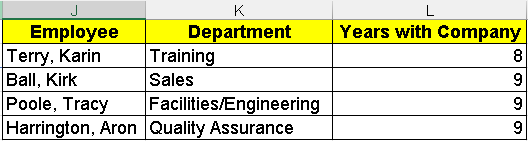
=VLOOKUP(J2,A:H,3,0)
where J2 is the Employee name which we need to lookup
A:H is the dataset
3 is the no of columns we need to look up at - here Department is the 3rd column from the right. 
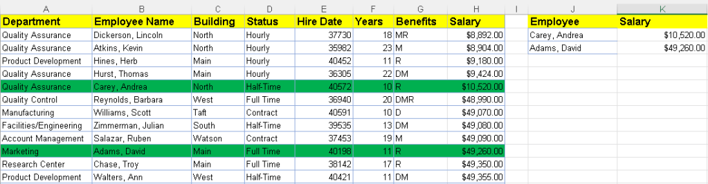
0 -Exact match 

Excel Function 8 – Use the MATCH() and INDEX() functions

We were using V-lookup and H-lookup to find our desired value earlier. And as long as the lookup value is in the first column or the first row of your data, those two will work just fine. 

However, a lot of times our data is not laid out in that manner, and if that’s the case then match and index are the functions that you’ll want to try and use. We will use match to find the row number on which our value resides. 

Once we have completed that match function, we will cut the function and actually paste it right into the row value in the index function. The index function will then return the value that it finds on that particular row that was found by the match function and it will base it on the column number or the array that we enter into the formula. So we’ll be creating match and then nesting it right inside of index.

Confused right? Lets see with an example.

If I need to find the salary of Andrea and David, the formula goes like this.

INDEX(array, row_num, [column_num])

=INDEX(A1:H736,MATCH(J2,B:B,0),MATCH(K1,A1:H1,0))

where A1:H736 is the complete data set

row number will the employee name so used Match. 

Salary will the column name so used Match function again. 

MATCH(lookup_value, lookup_array, [match_type])

To fetch the employee name, MATCH(J2,B:B,0)
J2 -  Employee reference
B:B is the column name referrig to Employee data

To fetch the salary details for the reference employee, MATCH(K1,A1:H1,0)

K1 is the column filed name "Salary"
A1:H1 is the array of all the column names. 

Excel Function 9 – DATE() functions

Teh four date functions which we are going to see is

• NOW()
• TODAY()
• WEEKDAY()
• WORKDAY()
• Networkdays()

NOW() & TODAY()

NOW formula in Excel displays the current time as a time serial number. Very useful Functions in Excel that take no arguments at all.

=TODAY()

=NOW()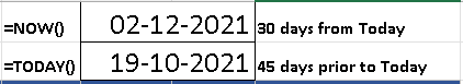

=NOW()+DAY(30)

=TODAY()-DAY(45)

WORKDAY() & WEEKDAY()

Workday(), returns a date n working days in the future or past.

=WORKDAY (start_date, days, [holidays])

• start_date – The date from which to start.
• days – The working days before or after start_date.
• holidays – [optional] A list dates that should be considered non-work days.

=WORKDAY("4-JUN-2021",1,F5:F13)// returns 7-JUN-2021
1 IS THE DAY
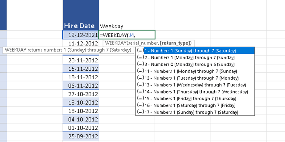
f5:f13 is the holidays list which i saturday and sumday. 

=WEEKDAY(serial_number,[return_type])

1. Serial_number (required argument) – This is a sequential number representing the date of the day that we are trying to find.
2. Return_type (optional argument) – This specifies which integers are to be assigned to each weekday. Possible values are:

Networkdays function – The NETWORKDAYS function returns the number of weekdays (weekends excluded) between two dates.

NETWORKDAYS()

=NETWORKDAYS (start_date, end_date, [holidays])

• start_date – The start date.
• end_date – The end date.
• holidays – [optional] A list of non-work days as dates.

Excel Function 10- CONSOLIDATE FUNCTION

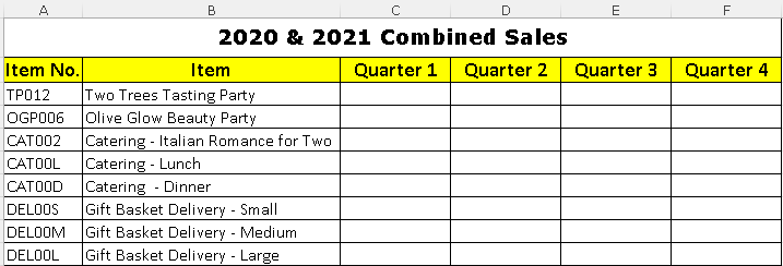
The consolidate function in Excel allows one to combine information from multiple workbooks into one place.  The Excel consolidate function lets you select data from its various locations and creates a table to summarize the information for you.

Say I have two excel sheets with same number of column headings and same format of data as below:

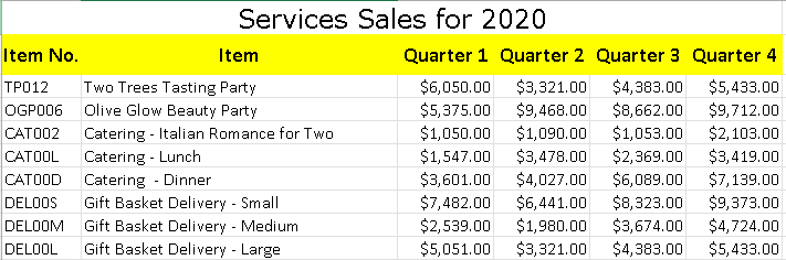
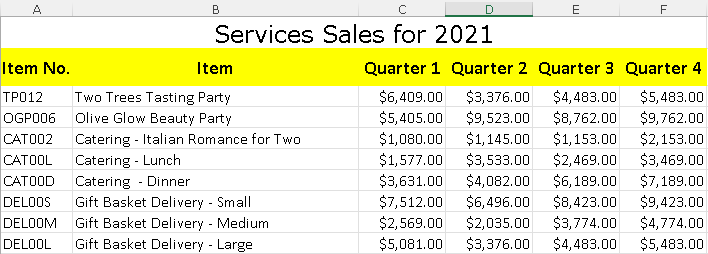
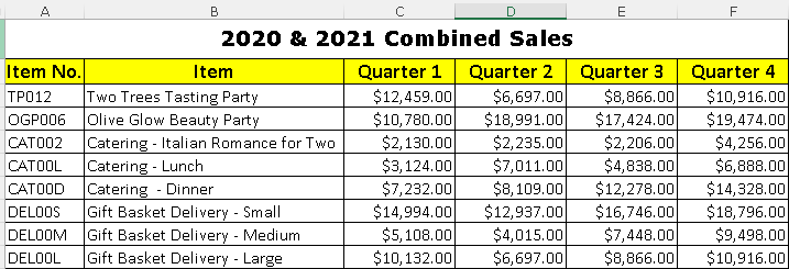
I can use consolidate function as below to find the combined sales.

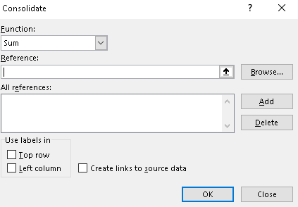
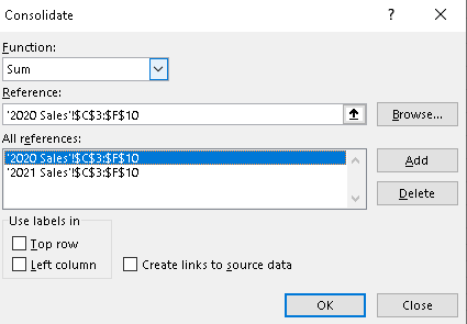
Go to Data menu, click consolidate. The below dialog box opens up.

Hope you found the post informative. Your valuable feedback, question, or comments about this post are always welcome by leaving me message on  contact form is truly appreciated.